Diffusion：[NeurIPS 2020] DDPM

Denoising Diffusion Probabilistic Models (DDPM)

作者: Jonathan Ho, Ajay Jain, Pieter Abbeel
机构: UC Berkeley
会议: NeurIPS 2020
版本: arXiv v2（2020-12-16；v1 2020-06-19）
链接: arXiv · NeurIPS · Code

一句话总结

DDPM 固定一条逐步加入高斯噪声的前向马尔可夫链，并训练时间条件 U-Net 预测噪声，从标准高斯经 1000 次反向去噪生成图像。

核心贡献

1. 高质量扩散生成: 证明 diffusion probabilistic model 能在无条件 CIFAR10 上达到 FID 3.17、IS 9.46，并扩展到 256×256 图像。
2. 噪声预测参数化: 把反向高斯均值改写为 ε prediction，显式连接变分推断、denoising score matching 与 Langevin-like sampling。
3. 简化训练目标: 提出去除 ELBO 时间步权重的 L_simple，以略差的 NLL 换取显著更好的感知样本质量与训练稳定性。
4. 渐进解码解释: 从 rate–distortion 和自回归广义位序角度解释反向链为何先恢复全局结构、后补高频细节，同时明确压缩算法只是概念证明。

📖 批读导航

Section	内容
00 - Abstract	机制主张、关键结果与证据边界
01 - Introduction	扩散模型问题设定与论文贡献
02 - Background	前向/反向过程、闭式加噪与 ELBO 分解
03 - Method	ε prediction、L_simple、训练与采样算法
04 - Experiments	样本质量、消融、渐进编码与插值
05 - Related Work	DDPM 与 NCSN、VAE、flow、EBM 的关系
06 - Conclusion & Impact	贡献、适用边界与社会影响
07 - Appendix A	ELBO 与边缘 KL 的逐步推导
08 - Appendix B	架构、超参数、训练与采样成本
09 - Appendix D	未筛选样本、最近邻与 coarse-to-fine 证据

关键数字

指标	数值
CIFAR10 FID / IS	3.17 / 9.46±0.11（无条件，L_simple；FID 相对训练集）
CIFAR10 NLL	≤3.75 bits/dim（L_simple）对 ≤3.70（原始 ELBO、固定方差）
扩散步数	T=1000；β 从 10⁻⁴ 线性增加到 0.02
LSUN Bedroom FID	4.90（约 256M 参数大模型）；小模型 6.36
原论文采样成本	CIFAR10 256 张约 17 秒；256² 图像 128 张约 300 秒（TPU v3-8）

方法概览

$$\text{训练:}\quad x_0,\; t,\; \epsilon \longrightarrow x_t = \sqrt{\bar{\alpha}_t}\,x_0 + \sqrt{1-\bar{\alpha}_t}\,\epsilon \longrightarrow \epsilon_\theta(x_t,t) \longrightarrow \left\lVert \epsilon-\epsilon_\theta(x_t,t) \right\rVert_2^2$$

$$\text{采样:}\quad x_T \sim \mathcal{N}(0,I),\qquad x_t \xrightarrow{\epsilon_\theta(x_t,t)} x_{t-1} \quad (t=T,\ldots,1) \longrightarrow x_0$$

训练可直接构造任意时间步的 $x_t$，因此每个 batch 只需一次网络前向；采样必须严格从 $T$ 到 1 串行执行。由 $\epsilon_\theta$ 得到反向均值后，再按固定 $\sigma_t^2$ 采样 $x_{t-1}$，最后一步不再加噪。

与相关方法对比

方案	预测/优化对象	采样机制	主要权衡
DDPM + 原始 ELBO	加权高斯 KL；可预测后验均值或 ε	1000 步随机反向马尔可夫链	更好 NLL，但感知质量较弱
DDPM + L_simple	各时间步未加权的 ε-MSE	同一条 1000 步反向链	FID 最佳但不是严格等权 ELBO
NCSN	多噪声级 score matching	训练后配置 annealed Langevin sampler	采样系数与训练目标的耦合较弱
自回归模型	逐坐标条件似然	按固定顺序串行解码	似然强；位序与每步可见上下文受限

📊 Citation Landscape

数据快照：Semantic Scholar，2026-08-13。引用数字会随时间变化。

TLDR (Semantic Scholar): High quality image synthesis results are presented using diffusion probabilistic models, a class of latent variable models inspired by considerations from nonequilibrium thermodynamics, which naturally admit a progressive lossy decompression scheme that can be interpreted as a generalization of autoregressive decoding.

引用统计: 参考文献 73 篇 | 被引 33,946 次 | Influential Citations: 4,828

参考文献分组 (Top 5 per category, by citations)

扩散与变分建模基础

论文	年份	引用
Auto-Encoding Variational Bayes	2013	16,817
Deep Unsupervised Learning using Nonequilibrium Thermodynamics	2015	10,525
A Connection Between Score Matching and Denoising Autoencoders	2011	2,296

Score、能量模型与采样

论文	年份	引用
Generative Modeling by Estimating Gradients of the Data Distribution	2019	5,852
Improved Techniques for Training Score-Based Generative Models	2020	1,500
Your Classifier is Secretly an Energy Based Model and You Should Treat it Like One	2019	671

架构与生成评测

论文	年份	引用
U-Net: Convolutional Networks for Biomedical Image Segmentation	2015	99,795
GANs Trained by a Two Time-Scale Update Rule Converge to a Local Nash Equilibrium	2017	19,274
Group Normalization	2018	4,513
PixelCNN++: Improving the PixelCNN with Discretized Logistic Mixture Likelihood and Other Modifications	2017	1,045

推荐论文（Semantic Scholar Recommendations）

论文	年份	方向	arXiv
Probing Diffusion Denoising Dynamics for Contrastive Representation Learning	2026	研究逐步去噪动态中表征何时形成	2607.09067
On the Redundancy of Timestep Embeddings in Diffusion Models	2026	检验 DDPM 时间条件设计是否存在冗余	2606.20416
Robust Diffusion Models via Divergence-Induced Weighted Denoising	2026	重新设计噪声预测的时间步加权以提高稳健性	2606.22521
ZeroGVC: Zero-Shot Generative Video Compression with Autoregressive Diffusion Priors	2026	延伸 DDPM 的生成压缩与自回归解码解释	2606.22371

🔗 相关链接

• arXiv
• NeurIPS Proceedings
• Official code
• Semantic Scholar

Denoising Diffusion Probabilistic Models

📌 预览

论文研究能否把图像逐步加噪，再学习逆转这一过程，从而得到能与当时强 GAN 竞争的生成模型。第一次阅读只需抓住“固定加噪、学习去噪”；变分下界、score matching 和 Langevin dynamics 的严格关系留到 Method。

Jonathan Ho · Ajay Jain · Pieter Abbeel

UC Berkeley

Abstract

💡 研究问题: DDPM 不是普通的图像去噪器，而是一个生成模型：它要从随机噪声出发，通过许多小的去噪步骤生成新图像。论文要验证的是，这种多步生成方式能否达到高质量图像合成的水平。

We present high quality image synthesis results using diffusion probabilistic models, a class of latent variable models inspired by considerations from nonequilibrium thermodynamics. Our best results are obtained by training on a weighted variational bound designed according to a novel connection between diffusion probabilistic models and denoising score matching with Langevin dynamics, and our models naturally admit a progressive lossy decompression scheme that can be interpreted as a generalization of autoregressive decoding. On the unconditional CIFAR10 dataset, we obtain an Inception score of 9.46 and a state-of-the-art FID score of 3.17. On 256x256 LSUN, we obtain sample quality similar to ProgressiveGAN. Our implementation is available at https://github.com/hojonathanho/diffusion.

💡 模型是什么: $x_0$ 是真实图像，$x_1,\ldots,x_T$ 是逐渐变吵的中间状态，$x_T$ 最终接近高斯噪声。前向过程固定，负责制造训练样本；反向过程由神经网络学习，负责生成图像。

训练：真实图像 x₀ ──逐步加噪──→ x_T ≈ 高斯噪声
生成：高斯噪声 x_T ──逐步去噪──→ x₀

💡 训练目标: 变分下界把整体生成目标拆成各时间步的去噪任务；作者进一步将其简化为预测所加噪声 $\epsilon$ 的均方误差。这个目标也可从 denoising score matching 理解，而逐步采样则类似 Langevin dynamics。三者是对同一个反向过程的不同解释，不是三套算法。

💡 渐进解码: 反向过程通常先形成整体结构，再补充细节，因此中间状态可看作质量逐步提高的解码结果。与自回归模型逐像素生成不同，DDPM 每一步都更新整张图像。

💡 结果与边界:

• 无条件 CIFAR-10：Inception Score 9.46，FID 3.17；后者是当时最佳结果。
• LSUN 256×256：样本质量与 ProgressiveGAN 相近。
• 这些结果说明 DDPM 的生成质量具有竞争力，但不代表采样快；原始 DDPM 仍需串行执行大量去噪步骤。

🔖 Section 总结

DDPM 固定一条逐步加噪的前向链，再学习反向去噪链，把从噪声生成图像的问题拆成许多较小的去噪任务。噪声预测目标连接了变分推断、score matching 与 Langevin 采样，并带来了当时很强的无条件图像生成结果。

核心洞察

1. 前向过程负责加噪，反向过程负责生成；真正需要学习的是反向过程。
2. 网络最终预测噪声 $\epsilon$，而不是直接一次生成完整图像。
3. CIFAR-10 上的 FID 3.17 是摘要最强的定量证据，LSUN 上只声称与 ProgressiveGAN 相近。
4. DDPM 用多步串行采样换取高生成质量。

1 Introduction

📌 预览

本节先把 DDPM 放回 2020 年的生成模型版图：当时 GAN、autoregressive model、flow 和 VAE 已能生成高质量样本，score-based model 也开始接近 GAN，但 diffusion probabilistic model 还没有证明自己能生成好图像。作者随后给出论文的三条主线：用许多小高斯去噪步骤构造生成链、用一种与 score matching / Langevin dynamics 相连的参数化改善样本质量，以及用渐进解码解释“样本好看但似然不强”的现象。

Deep generative models of all kinds have recently exhibited high quality samples in a wide variety of data modalities. Generative adversarial networks (GANs), autoregressive models, flows, and variational autoencoders (VAEs) have synthesized striking image and audio samples [14, 27, 3, 58, 38, 25, 10, 32, 44, 57, 26, 33, 45], and there have been remarkable advances in energy-based modeling and score matching that have produced images comparable to those of GANs [11, 55].

💡 **研究背景：**几条主流路线已经各有优势与代价：

路线	生成方式	当时的突出特点	常见代价
GAN	一次前向映射：噪声 $z\rightarrow x$	样本锐利、生成快	没有显式似然，训练可能不稳定或模式覆盖不足
Autoregressive	按顺序生成像素 / token	显式似然强、分解清楚	生成必须串行
Normalizing flow	可逆变换：$z\leftrightarrow x$	精确似然、可逆	架构受可逆性约束
VAE	潜变量编码与解码	变分推断稳定、潜空间明确	当时常见图像偏平滑
Score-based model	学习 $\nabla_x\log p(x)$，再迭代采样	已展示接近 GAN 的质量	采样同样需要多步迭代

DDPM 的目标，是把潜变量概率模型的训练框架与score-based 迭代生成的样本质量连接起来。

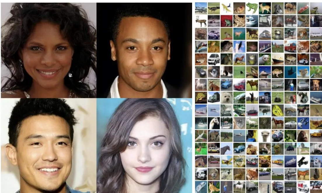
Figure 1: Generated samples on CelebA-HQ 256 × 256 (left) and unconditional CIFAR10 (right)

💡 Figure 1｜先展示“它能生成什么”:

• 左侧是 $256\times256$ 的 CelebA-HQ 人脸，右侧是 $32\times32$ 的 CIFAR-10 自然图像；两者分辨率与数据复杂度不同，不能凭肉眼横向判断哪个任务做得更好。
• CIFAR-10 结果是 unconditional generation：采样时不提供类别标签，模型既要决定生成什么类别，也要生成其外观。
• 图中可看到人脸的整体一致性，以及 CIFAR-10 中动物、车辆等多种语义，但这仍只是经过展示的有限样本。它能证明模型具有生成能力，却不能单独证明分布覆盖、非记忆性或相对基线优势；这些需要后文 FID、Inception Score 和 nearest-neighbor 分析支持。

This paper presents progress in diffusion probabilistic models [53]. A diffusion probabilistic model (which we will call a “diffusion model” for brevity) is a parameterized Markov chain trained using variational inference to produce samples matching the data after finite time. Transitions of this chain are learned to reverse a diffusion process, which is a Markov chain that gradually adds noise to the data in the opposite direction of sampling until signal is destroyed. When the diffusion consists of small amounts of Gaussian noise, it is sufficient to set the sampling chain transitions to conditional Gaussians too, allowing for a particularly simple neural network parameterization.

💡 模型定义:

• $x_0$ 是真实图像，$x_1,\ldots,x_{T-1}$ 是与图像同形状的潜变量，$x_T$ 接近标准高斯噪声。
• 前向过程 $q(x_t\mid x_{t-1})$ 每次只加少量高斯噪声。它负责把复杂、未知的数据分布逐渐变成简单、已知的噪声分布；在本文实现中，这条链不由神经网络学习。
• 反向过程 $p_\theta(x_{t-1}\mid x_t)$ 从噪声出发，每次恢复一点信号。参数 $\theta$ 属于带时间条件的神经网络，这才是训练要学习的部分。
• “Markov” 表示每一步只依赖相邻状态：给定 $x_t$ 后，生成 $x_{t-1}$ 不需要再显式查看更早的 $x_{t+1},\ldots,x_T$。

为什么小步加噪很重要？ 如果一步就把图像变成纯噪声，逆问题会极度多解；拆成许多足够小的步骤后，相邻分布只发生局部变化，反向条件分布可以用高斯近似，并由神经网络预测其均值。这是 DDPM 用较长采样链换取简单单步建模的核心交易。

Figure 2: The directed graphical model considered in this work.

💡 Figure 2: 噪声 $x_T$ 放在左边、数据 $x_0$ 放在右边，所以：

前向 / 加噪 q：x₀ → x₁ → … → xₜ₋₁ → xₜ → … → x_T     （图中虚线向左）
反向 / 生成 pθ：x_T → … → xₜ → xₜ₋₁ → … → x₁ → x₀     （图中实线向右）

图中的实线 $p_\theta(x_{t-1}\mid x_t)$ 是生成时真正执行的方向；虚线 $q(x_t\mid x_{t-1})$ 是训练时用真实图像构造带噪样本的方向。两条链经过相同的状态层级，但条件概率方向相反。

训练数据只直接提供 $x_0$，中间状态都是潜变量。作者用已知的前向链 $q$ 充当近似后验，并优化一个可计算的 variational bound，让学习到的反向链 $p_\theta$ 逼近真实逆过程。下一章会把这个整体目标分解成每个时间步之间的 KL divergence；此处先把它理解为：用已知加噪过程制造监督信号，逐步教会模型如何逆转它。

Diffusion models are straightforward to define and efficient to train, but to the best of our knowledge, there has been no demonstration that they are capable of generating high quality samples. We show that diffusion models actually are capable of generating high quality samples, sometimes better than the published results on other types of generative models (Section 4). In addition, we show that a certain parameterization of diffusion models reveals an equivalence with denoising score matching over multiple noise levels during training and with annealed Langevin dynamics during sampling (Section 3.2) [55, 61]. We obtained our best sample quality results using this parameterization (Section 4.2), so we consider this equivalence to be one of our primary contributions.

💡 论文推进了什么: 扩散模型的基本框架来自更早的工作 [53]；DDPM 的贡献不是首次提出“逐步加噪再反演”，而是证明这类模型可以产生高质量图像，并找到一种效果很好的反向过程参数化。后文会让网络预测加入 $x_0$ 的噪声 $\epsilon$，再把预测结果转换成反向高斯的均值。

这一参数化把训练和采样连接到同一个量——噪声尺度 $t$ 下的 score：

$$\nabla_{x_t}\log q_t(x_t),$$

即“在当前位置向哪个方向移动，概率密度上升得最快”。训练时，denoising score matching 借助已知加噪样本学习这片方向场；采样时，annealed Langevin dynamics 从高噪声开始，沿学到的方向移动并保留适量随机性，再逐渐降低噪声尺度。严格的比例关系和损失推导在 Section 3.2 才会出现，这里先记住：

ε-prediction（网络输出）
         ↕ 可换算
score（概率密度上升方向）
         ↓ 用于
Langevin-like reverse sampling（逐步生成）

Section 4.2 通过预测 $\epsilon$ 与预测后验均值 $\tilde\mu_t$ 的消融实验来验证。

Despite their sample quality, our models do not have competitive log likelihoods compared to other likelihood-based models (our models do, however, have log likelihoods better than the large estimates annealed importance sampling has been reported to produce for energy based models and score matching [11, 55]). We find that the majority of our models’ lossless codelengths are consumed to describe imperceptible image details (Section 4.3). We present a more refined analysis of this phenomenon in the language of lossy compression, and we show that the sampling procedure of diffusion models is a type of progressive decoding that resembles autoregressive decoding along a bit ordering that vastly generalizes what is normally possible with autoregressive models.

💡 为什么“图像好看”与“似然不强”可以同时成立:

• FID / 人眼观感更关注样本是否具有真实图像的语义与感知统计，例如物体轮廓、纹理和多样性。
• log likelihood要求模型给每一张真实图像的每个精确像素配置高概率；换成无损编码语言，负对数似然越低，理论码长越短。
• DDPM 的变分目标把大量码长用在了人眼几乎察觉不到的细节上。模型可能生成很自然的图像，却在精确复现这些微小像素变化时付出较高码长，因此似然排名落后。

这不是说似然“没有用”，而是说明两种指标奖励的内容不同：感知质量关心哪些差异重要，严格似然把每个可编码差异都计入。 作者使用重加权训练目标改善样本质量，也意味着不能期待它同时把原始 likelihood bound 优化到最好。

💡 渐进解码｜第三种理解反向链的方式: 在自回归模型里，解码通常沿固定坐标顺序逐像素或逐 token 展开；在扩散模型里，每个反向时间步都同时更新整张图像，早期形成粗略全局信息，后期逐渐加入精细信息。中间状态因而可以被看作同一幅图像从低码率、低保真到高码率、高保真的渐进重建。

自回归：已生成区域逐步扩大      [局部坐标顺序]
扩散模型：整幅图像逐步变清晰    [噪声尺度顺序]

“generalization of autoregressive decoding” 指的是解码顺序不再局限于一个预定的像素排列，而不是说 DDPM 在似然或速度上自动优于自回归模型。Section 4.3 会用率失真曲线检验这个解释。

🧭 Introduction:

生成模型已经能合成高质量图像
                ↓
但 diffusion model 尚未证明自己的样本质量
                ↓
小步高斯扩散让反向条件分布易于参数化
                ↓
ε-prediction 连接变分训练、score matching 与 Langevin-like 采样
                ↓
实验检验高样本质量；压缩视角解释似然短板与渐进生成

🔖 Section 总结

Introduction 把 DDPM 定位为一项“让已有扩散框架真正生成出高质量图像”的工作。其基本策略是把困难的一步生成拆成许多局部高斯去噪步骤，再通过噪声预测参数化把变分概率模型、denoising score matching 与 Langevin-like sampling 连接起来。作者也主动暴露了核心权衡：模型的感知样本质量很强，但严格 log likelihood 不具竞争力；渐进有损解码提供了解释这一差异的视角。

核心洞察

1. DDPM 的历史贡献不是发明扩散过程本身，而是找到有效参数化和训练目标，首次有力证明扩散模型能生成高质量图像。
2. 小步高斯加噪把一个高度多解的逆问题拆成许多较简单的局部逆问题；代价是生成必须串行经过很多时间步。
3. 前向链 $q$ 负责构造带噪训练样本，反向链 $p_\theta$ 才负责生成。
4. 噪声预测、score learning 和 Langevin-like sampling 是同一机制在网络输出、概率几何和采样算法三个层面的表达。
5. 较优 FID 与较差 likelihood 并不矛盾：前者偏向感知结构，后者还会惩罚模型未能精确编码的人眼不可见细节。

2 Background

📌 预览

本节定义 DDPM 的两条马尔可夫链：学习从噪声生成数据的反向过程 $p_\theta$，用固定的前向过程 $q$ 构造训练监督。阅读重点是三步：前向过程如何闭式采样任意 $x_t$，变分上界如何拆成逐步 KL，以及真实单步后验如何解析求出。

Diffusion models [53] are latent variable models of the form $p_\theta(\mathbf{x}_0):=\int p_\theta(\mathbf{x}_{0:T})\,d\mathbf{x}_{1:T}$, where $\mathbf{x}_1,\ldots,\mathbf{x}_T$ are latents of the same dimensionality as the data $\mathbf{x}_0\sim q(\mathbf{x}_0)$. The joint distribution $p_\theta(\mathbf{x}_{0:T})$ is called the reverse process, and it is defined as a Markov chain with learned Gaussian transitions starting at $p(\mathbf{x}_T)=\mathcal{N}(\mathbf{x}_T;\mathbf{0},\mathbf{I})$

$$p_\theta(\mathbf{x}_{0:T}) :=p(\mathbf{x}_T)\prod_{t=1}^{T}p_\theta(\mathbf{x}_{t-1}\mid\mathbf{x}_t), \qquad p_\theta(\mathbf{x}_{t-1}\mid\mathbf{x}_t) :=\mathcal{N}\!\left(\mathbf{x}_{t-1}; \boldsymbol{\mu}_\theta(\mathbf{x}_t,t), \boldsymbol{\Sigma}_\theta(\mathbf{x}_t,t)\right). \tag{1}$$

💡 式 (1)｜反向生成链:

第一步：

模型最终需要的是 $p_\theta(x_0)$，即生成一张干净图像的概率。但生成过程包含整条隐变量路径 $x_T,x_{T-1},\ldots,x_1$，所以先写联合分布，再把中间变量积分掉：

$$p_\theta(\mathbf{x}_0) = \int p_\theta(\mathbf{x}_{0:T}) \,d\mathbf{x}_{1:T}.$$

第二步：

按概率链式法则，从 $x_T$ 向 $x_0$ 展开可得

$$p_\theta(\mathbf{x}_{0:T}) = p(\mathbf{x}_T) \prod_{t=1}^{T} p_\theta(\mathbf{x}_{t-1}\mid\mathbf{x}_{t:T}).$$

DDPM 进一步采用一阶马尔可夫假设：已知当前状态 $x_t$ 后，其余更高噪声状态 $x_{t+1:T}$ 不再提供额外信息。因此

$$p_\theta(\mathbf{x}_{t-1}\mid\mathbf{x}_{t:T}) = p_\theta(\mathbf{x}_{t-1}\mid\mathbf{x}_t),$$

于是得到式 (1) 的乘积形式：

$$p_\theta(\mathbf{x}_{0:T}) :=p(\mathbf{x}_T)\prod_{t=1}^{T}p_\theta(\mathbf{x}_{t-1}\mid\mathbf{x}_t)$$

第三步：

$$\qquad p_\theta(\mathbf{x}_{t-1}\mid\mathbf{x}_t) :=\mathcal{N}\!\left(\mathbf{x}_{t-1}; \boldsymbol{\mu}_\theta(\mathbf{x}_t,t), \boldsymbol{\Sigma}_\theta(\mathbf{x}_t,t)\right)$$

即：

$$\mathbf x_{t-1}\mid\mathbf x_t \sim \mathcal N\left( \boldsymbol\mu_\theta(\mathbf x_t,t), \boldsymbol\Sigma_\theta(\mathbf x_t,t) \right)$$

其中 $p_\theta(x_{t-1}\mid x_t)$ 被建模成高斯分布。神经网络接收当前带噪样本 $x_t$ 和时间步 $t$，输出：

• 均值 $\mu_\theta(x_t,t)$：这一步去噪后最可能到达的位置；
• 协方差 $\Sigma_\theta(x_t,t)$：这一步还应保留多少随机性。

因此生成过程可以直接从公式读出：先采样 $x_T\sim\mathcal N(0,I)$，再依次采样 $x_{T-1},x_{T-2},\ldots,x_0$。其中 $x_0,\ldots,x_T$ 都与原图同维，只是噪声程度不同。

What distinguishes diffusion models from other types of latent variable models is that the approximate posterior $q\big(\mathbf{x}_{1:T}\mid\mathbf{x}_0\big)$, called the forward process or diffusion process, is fixed to a Markov chain that gradually adds Gaussian noise to the data according to a variance schedule $\beta_1,\dots,\beta_T$:

$$q(\mathbf{x}_{1:T}\mid\mathbf{x}_0) :=\prod_{t=1}^{T}q(\mathbf{x}_t\mid\mathbf{x}_{t-1}), \qquad q(\mathbf{x}_t\mid\mathbf{x}_{t-1}) :=\mathcal{N}\!\left(\mathbf{x}_t; \sqrt{1-\beta_t}\,\mathbf{x}_{t-1}, \beta_t\mathbf{I}\right). \tag{2}$$

💡 式 (2)｜前向加噪:

先看一步转移。 令

$$\alpha_t:=1-\beta_t,$$

则式 (2) 表示

$$q(\mathbf{x}_t\mid\mathbf{x}_{t-1}) := \mathcal N\!\left( \sqrt{\alpha_t}\mathbf{x}_{t-1}, \beta_t\mathbf I \right).$$

从这个高斯采样，等价于：

$$\mathbf{x}_t = \sqrt{\alpha_t}\mathbf{x}_{t-1} + \sqrt{\beta_t}\boldsymbol{\epsilon}_t, \qquad \boldsymbol{\epsilon}_t\sim\mathcal N(\mathbf 0,\mathbf I).$$

$\mathbf I$ 是单位矩阵，表示各个维度加入相互独立、方差相同的噪声。

这里出现平方根，是因为系数 $c$ 乘在随机变量上时，方差会乘以 $c^2$：

• 旧信号的方差比例由 $\alpha_t$ 决定，所以幅度乘 $\sqrt{\alpha_t}$；
• 新噪声的方差是 $\beta_t$，所以标准差为 $\sqrt{\beta_t}$。

例如 $\beta_t=0.01$ 时，旧信号幅度乘 $\sqrt{0.99}\approx0.995$，同时加入标准差为 $0.1$ 的高斯噪声。单步变化很小，但重复很多次后，数据结构会逐渐被噪声覆盖。

随着 $t$ 增大，原始信号不断衰减；当累计信号保留比例接近于 $0$ 时，$x_t$ 的分布将近似标准正态分布 $\mathcal N(\mathbf 0,\mathbf I)$，这也解释了反向生成过程为什么从高斯噪声 $x_T$ 出发。

再看整条链。 给定 $x_0$ 后，每一步只依赖前一步，因此路径概率就是各步转移概率的乘积：

$$q(\mathbf{x}_{1:T}\mid\mathbf{x}_0) = q(\mathbf{x}_1\mid\mathbf{x}_0) q(\mathbf{x}_2\mid\mathbf{x}_1) \cdots q(\mathbf{x}_T\mid\mathbf{x}_{T-1}).$$

$q$ 是人为指定的加噪过程，不负责生成；它的作用是把训练图像变成不同噪声强度的样本，为反向链 $p_\theta$ 提供监督。

Training is performed by optimizing the usual variational bound on negative log likelihood:

$$\mathbb{E}\!\left[-\log p_\theta(\mathbf{x}_0)\right] \leq \mathbb{E}_q\!\left[-\log\frac{p_\theta(\mathbf{x}_{0:T})}{q(\mathbf{x}_{1:T}\mid\mathbf{x}_0)}\right] = \mathbb{E}_q\!\left[-\log p(\mathbf{x}_T) -\sum_{t\geq1}\log\frac{p_\theta(\mathbf{x}_{t-1}\mid\mathbf{x}_t)}{q(\mathbf{x}_t\mid\mathbf{x}_{t-1})}\right] =:L. \tag{3}$$

💡 式 (3)｜变分上界:

直接计算 $p_\theta(x_0)$ 需要积分掉 $x_{1:T}$，通常不可行。变分推导的作用，就是把这个难算的边缘概率变成一个可以沿前向过程 $q$ 采样估计的目标。

第一步：在积分中乘除同一个 $q$。

$$p_\theta(\mathbf{x}_0) = \int q(\mathbf{x}_{1:T}\mid\mathbf{x}_0) \frac{p_\theta(\mathbf{x}_{0:T})} {q(\mathbf{x}_{1:T}\mid\mathbf{x}_0)} \,d\mathbf{x}_{1:T}.$$

根据期望的定义，上式等于

$$p_\theta(\mathbf{x}_0) = \mathbb E_{q(\mathbf{x}_{1:T}\mid\mathbf{x}_0)} \left[ \frac{p_\theta(\mathbf{x}_{0:T})} {q(\mathbf{x}_{1:T}\mid\mathbf{x}_0)} \right].$$

第二步：使用 Jensen 不等式。

记

$$w = \frac{p_\theta(\mathbf{x}_{0:T})} {q(\mathbf{x}_{1:T}\mid\mathbf{x}_0)}.$$

训练的目标是最大化数据似然 $p_\theta(x_0)$，也就是最小化负对数似然 $-\log p_\theta(x_0)$。而 $p_\theta(x_0)=\mathbb E_q[w]$，即最小化 $-\log\mathbb E_q[w]$；利用 Jensen 不等式，可以进一步得到这一目标的可计算上界：

Jensen 不等式：

如果函数是凸函数：

$$f(\mathbb E[x])\leq \mathbb E[f(x)]$$

如果是凹函数：

$$f(\mathbb E[x])\geq \mathbb E[f(x)]$$

因为 $-\log$ 是凸函数，

$$-\log\mathbb E_q[w] \leq \mathbb E_q[-\log w].$$

代回 $w$，便得到式 (3) 的第一个不等号：

$$-\log p_\theta(\mathbf{x}_0) \leq \mathbb E_q \left[ -\log \frac{p_\theta(\mathbf{x}_{0:T})} {q(\mathbf{x}_{1:T}\mid\mathbf{x}_0)} \right].$$

第三步：展开两条马尔可夫链。

$$\frac{p_\theta(\mathbf{x}_{0:T})} {q(\mathbf{x}_{1:T}\mid\mathbf{x}_0)} = \frac{ p(\mathbf{x}_T) \prod_{t=1}^{T}p_\theta(\mathbf{x}_{t-1}\mid\mathbf{x}_t) }{ \prod_{t=1}^{T}q(\mathbf{x}_t\mid\mathbf{x}_{t-1}) }.$$

对乘积取 $-\log$ 后，乘法变加法、除法变减法：

$$-\log p(\mathbf{x}_T) - \sum_{t=1}^{T} \log \frac{ p_\theta(\mathbf{x}_{t-1}\mid\mathbf{x}_t) }{ q(\mathbf{x}_t\mid\mathbf{x}_{t-1}) }.$$

因此得到式 (3) ：

$$\mathbb{E}\!\left[-\log p_\theta(\mathbf{x}_0)\right] \leq \mathbb{E}_q\!\left[-\log\frac{p_\theta(\mathbf{x}_{0:T})}{q(\mathbf{x}_{1:T}\mid\mathbf{x}_0)}\right] = \mathbb{E}_q\!\left[-\log p(\mathbf{x}_T) -\sum_{t\geq1}\log\frac{p_\theta(\mathbf{x}_{t-1}\mid\mathbf{x}_t)}{q(\mathbf{x}_t\mid\mathbf{x}_{t-1})}\right] =:L. \tag{3}$$

$L$ 是负对数似然的上界，因此训练时最小化 $L$；等价地，$-L$ 是 $\log p_\theta(x_0)$ 的下界，即 ELBO。

The forward process variances $\beta_t$ can be learned by reparameterization [33] or held constant as hyperparameters, and expressiveness of the reverse process is ensured in part by the choice of Gaussian conditionals in $p_\theta(\mathbf{x}_{t-1}\mid\mathbf{x}_t)$, because both processes have the same functional form when $\beta_t$ are small [53]. A notable property of the forward process is that it admits sampling $\mathbf{x}_t$ at an arbitrary timestep $t$ in closed form: using the notation $\alpha_t:=1-\beta_t$ and $\bar{\alpha}_t:=\prod_{s=1}^{t}\alpha_s$, we have

$$q(\mathbf{x}_t\mid\mathbf{x}_0) =\mathcal{N}\!\left( \mathbf{x}_t; \sqrt{\bar{\alpha}_t}\,\mathbf{x}_0, (1-\bar{\alpha}_t)\mathbf{I} \right). \tag{4}$$

💡 式 (4)｜多步噪声的闭式合并:

式 (2) 只能从 $x_{t-1}$ 生成 $x_t$。式 (4) 更重要：它允许直接从原图 $x_0$ 生成任意时刻的 $x_t$。

当 $t=1$ 时，$\bar\alpha_1=\alpha_1$ 且 $1-\bar\alpha_1=\beta_1$，式 (4) 就是式 (2)，因此归纳的起点成立。

第一步：写出归纳假设。

假设经过 $t-1$ 步后已经有

$$\mathbf{x}_{t-1} = \sqrt{\bar\alpha_{t-1}}\mathbf{x}_0 + \sqrt{1-\bar\alpha_{t-1}}\boldsymbol{\epsilon}', \qquad \boldsymbol{\epsilon}'\sim\mathcal N(\mathbf{0},\mathbf I).$$

其中

$$\bar\alpha_{t-1} = \alpha_1\alpha_2\cdots\alpha_{t-1}$$

是前 $t-1$ 步累计保留下来的信号方差比例。

第二步：代入第 $t$ 步加噪公式。

由式 (2) 的重参数化形式，

$$\mathbf{x}_t = \sqrt{\alpha_t}\mathbf{x}_{t-1} + \sqrt{\beta_t}\boldsymbol{\epsilon}_t.$$

代入 $x_{t-1}$：

$$\mathbf{x}_t = \sqrt{\alpha_t\bar\alpha_{t-1}}\mathbf{x}_0 + \sqrt{\alpha_t(1-\bar\alpha_{t-1})}\boldsymbol{\epsilon}' + \sqrt{\beta_t}\boldsymbol{\epsilon}_t.$$

因为 $\bar\alpha_t=\alpha_t\bar\alpha_{t-1}$，第一项正好是 $\sqrt{\bar\alpha_t}x_0$。

第三步：合并两个独立高斯噪声。

$\epsilon'$ 与 $\epsilon_t$ 相互独立，所以它们的线性组合仍是高斯。总噪声方差为

$$\alpha_t(1-\bar\alpha_{t-1})+\beta_t.$$

利用 $\beta_t=1-\alpha_t$ 和 $\bar\alpha_t=\alpha_t\bar\alpha_{t-1}$：

$$\alpha_t(1-\bar\alpha_{t-1})+\beta_t = \alpha_t-\bar\alpha_t+1-\alpha_t = 1-\bar\alpha_t.$$

因而两个噪声项可以合写成一个新的标准高斯 $\epsilon$：

$$\mathbf{x}_t = \sqrt{\bar\alpha_t}\mathbf{x}_0 + \sqrt{1-\bar\alpha_t}\boldsymbol{\epsilon}, \qquad \boldsymbol{\epsilon}\sim\mathcal N(\mathbf{0},\mathbf I).$$

这就是式 (4)。$\bar\alpha_t$ 越小，保留的原图越少；对应的信噪比为

$$\operatorname{SNR}(t) = \frac{\bar\alpha_t}{1-\bar\alpha_t}.$$

训练意义： 随机抽到时间步 $t$ 后，只需采一个 $\epsilon$ 就能一步得到 $x_t$，不必真的执行 $t$ 次前向加噪。

Efficient training is therefore possible by optimizing random terms of $L$ with stochastic gradient descent. Further improvements come from variance reduction by rewriting $L$ (3) as:

$$\mathbb{E}_q\!\left[ \underbrace{D_{\mathrm{KL}}\!\left(q(\mathbf{x}_T\mid\mathbf{x}_0)\parallel p(\mathbf{x}_T)\right)}_{L_T} +\sum_{t>1} \underbrace{D_{\mathrm{KL}}\!\left(q(\mathbf{x}_{t-1}\mid\mathbf{x}_t,\mathbf{x}_0)\parallel p_\theta(\mathbf{x}_{t-1}\mid\mathbf{x}_t)\right)}_{L_{t-1}} +\underbrace{-\log p_\theta(\mathbf{x}_0\mid\mathbf{x}_1)}_{L_0} \right]. \tag{5}$$

💡 式 (3) → 式 (5)：把“整条路径比较”改写成“每一步去噪都学对”

式 (3) 里面出现的是

$$\frac{ p_\theta(\mathbf{x}_{t-1}\mid \mathbf{x}_t) }{ q(\mathbf{x}_t\mid \mathbf{x}_{t-1}) }$$

分子是反向过程：

$$\mathbf{x}_t\rightarrow \mathbf{x}_{t-1},$$

分母却是前向过程：

$$\mathbf{x}_{t-1}\rightarrow \mathbf{x}_t.$$

所以它还不能直接解释成“模型预测和正确答案之间的差距”。

我们真正想比较的是：

$$q(\mathbf{x}_{t-1}\mid \mathbf{x}_t,\mathbf{x}_0) \quad\text{和}\quad p_\theta(\mathbf{x}_{t-1}\mid \mathbf{x}_t)$$

其中：

$$q(\mathbf{x}_{t-1}\mid \mathbf{x}_t,\mathbf{x}_0)$$

表示已知当前噪声状态 $\mathbf{x}_t$，并且训练时还知道真实原图 $\mathbf{x}_0$，那么前一步 $\mathbf{x}_{t-1}$ 真正应该服从什么分布。

而

$$p_\theta(\mathbf{x}_{t-1}\mid \mathbf{x}_t)$$

则是模型预测出来的反向分布。

第一步：先把 $t=1$ 单独拿出来

$$L = \mathbb E_q \left[ -\log p(\mathbf{x}_T) - \sum_{t=1}^{T} \log \frac{ p_\theta(\mathbf{x}_{t-1}\mid\mathbf{x}_t) }{ q(\mathbf{x}_t\mid\mathbf{x}_{t-1}) } \right]$$

开始，把 $t=1$ 从求和里拆出来：

$$\begin{aligned} L = \mathbb E_q\Bigg[ &-\log p(\mathbf{x}_T) -\sum_{t=2}^{T} \log \frac{ p_\theta(\mathbf{x}_{t-1}\mid\mathbf{x}_t) }{ q(\mathbf{x}_t\mid\mathbf{x}_{t-1}) } - \log \frac{ p_\theta(\mathbf{x}_0\mid\mathbf{x}_1) }{ q(\mathbf{x}_1\mid\mathbf{x}_0) } \Bigg]. \end{aligned}$$

最后这一项展开为

$$-\log p_\theta(\mathbf{x}_0\mid\mathbf{x}_1) + \log q(\mathbf{x}_1\mid\mathbf{x}_0).$$

其中第一部分

$$\boxed{ -\log p_\theta(\mathbf{x}_0\mid\mathbf{x}_1) }$$

之后就会成为式 (5) 里的重建项 $L_0$。

第二步：把前向转移改写成“反向后验”

现在看中间任意一个 $t>1$。

原来出现的是：

$$q(\mathbf{x}_t\mid\mathbf{x}_{t-1}),$$

但我们想要的是：

$$q(\mathbf{x}_{t-1}\mid\mathbf{x}_t,\mathbf{x}_0).$$

这时利用 Bayes 公式。

在给定 $\mathbf{x}_0$ 的条件下，

$$q(\mathbf{x}_{t-1},\mathbf{x}_t\mid\mathbf{x}_0)$$

可以按两个方向分解。

按前向方向：

$$q(\mathbf{x}_{t-1},\mathbf{x}_t\mid\mathbf{x}_0) = q(\mathbf{x}_t\mid\mathbf{x}_{t-1}) q(\mathbf{x}_{t-1}\mid\mathbf{x}_0).$$

按后验方向：

$$q(\mathbf{x}_{t-1},\mathbf{x}_t\mid\mathbf{x}_0) = q(\mathbf{x}_{t-1}\mid\mathbf{x}_t,\mathbf{x}_0) q(\mathbf{x}_t\mid\mathbf{x}_0).$$

所以：

$$q(\mathbf{x}_t\mid\mathbf{x}_{t-1}) q(\mathbf{x}_{t-1}\mid\mathbf{x}_0) = q(\mathbf{x}_{t-1}\mid\mathbf{x}_t,\mathbf{x}_0) q(\mathbf{x}_t\mid\mathbf{x}_0).$$

整理得到：

$$\boxed{ q(\mathbf{x}_t\mid\mathbf{x}_{t-1}) = q(\mathbf{x}_{t-1}\mid\mathbf{x}_t,\mathbf{x}_0) \frac{ q(\mathbf{x}_t\mid\mathbf{x}_0) }{ q(\mathbf{x}_{t-1}\mid\mathbf{x}_0) } }$$

第三步：代回式 (3)

对任意 $t>1$：

$$-\log \frac{ p_\theta(\mathbf{x}_{t-1}\mid\mathbf{x}_t) }{ q(\mathbf{x}_t\mid\mathbf{x}_{t-1}) }$$

代入上面的 Bayes 结果：

$$-\log \frac{ p_\theta(\mathbf{x}_{t-1}\mid\mathbf{x}_t) }{ q(\mathbf{x}_{t-1}\mid\mathbf{x}_t,\mathbf{x}_0) \dfrac{ q(\mathbf{x}_t\mid\mathbf{x}_0) }{ q(\mathbf{x}_{t-1}\mid\mathbf{x}_0) } }.$$

整理后得到：

$$\log \frac{ q(\mathbf{x}_{t-1}\mid\mathbf{x}_t,\mathbf{x}_0) }{ p_\theta(\mathbf{x}_{t-1}\mid\mathbf{x}_t) } + \log \frac{ q(\mathbf{x}_t\mid\mathbf{x}_0) }{ q(\mathbf{x}_{t-1}\mid\mathbf{x}_0) }$$

现在已经出现了我们真正想要的第一项：

$$\log \frac{ q(\mathbf{x}_{t-1}\mid\mathbf{x}_t,\mathbf{x}_0) }{ p_\theta(\mathbf{x}_{t-1}\mid\mathbf{x}_t) }.$$

它就是 KL divergence 里面的标准 log-ratio。

第四步：剩下的边缘概率会自动消掉

除了刚才的 KL 部分之外，还剩：

$$\log \frac{ q(\mathbf{x}_t\mid\mathbf{x}_0) }{ q(\mathbf{x}_{t-1}\mid\mathbf{x}_0) } = \log q(\mathbf{x}_t\mid\mathbf{x}_0) - \log q(\mathbf{x}_{t-1}\mid\mathbf{x}_0).$$

再加上 $t=1$ 项里留下来的：

$$\log q(\mathbf{x}_1\mid\mathbf{x}_0).$$

全部加起来：

$$\begin{aligned} &\log q(\mathbf{x}_1\mid\mathbf{x}_0) \\ &+ \left[ \log q(\mathbf{x}_2\mid\mathbf{x}_0) - \log q(\mathbf{x}_1\mid\mathbf{x}_0) \right] \\ &+ \left[ \log q(\mathbf{x}_3\mid\mathbf{x}_0) - \log q(\mathbf{x}_2\mid\mathbf{x}_0) \right] \\ &+\cdots \\ &+ \left[ \log q(\mathbf{x}_T\mid\mathbf{x}_0) - \log q(\mathbf{x}_{T-1}\mid\mathbf{x}_0) \right]. \end{aligned}$$

中间所有项都会一正一负抵消：

$$\log q(\mathbf{x}_1\mid\mathbf{x}_0), \ldots, \log q(\mathbf{x}_{T-1}\mid\mathbf{x}_0)$$

全部消失，只剩：

$$\log q(\mathbf{x}_T\mid\mathbf{x}_0)$$

于是它和原来的

$$-\log p(\mathbf{x}_T)$$

合并成：

$$\log \frac{ q(\mathbf{x}_T\mid\mathbf{x}_0) }{ p(\mathbf{x}_T) }.$$

第五步：把这些 log-ratio 识别成 KL

KL divergence 的定义是：

$$D_{\mathrm{KL}}(q\parallel p) = \mathbb E_q \left[ \log\frac{q}{p} \right].$$

$$L = \mathbb E_q \left[ L_T + \sum_{t=2}^{T}L_{t-1} + L_0 \right]$$

其中三个部分分别是：

$$L_T = D_{\mathrm{KL}} \left( q(x_T\mid x_0) \parallel p(x_T) \right)$$

$$L_{t-1} = D_{\mathrm{KL}} \left( q(x_{t-1}\mid x_t,x_0) \parallel p_\theta(x_{t-1}\mid x_t) \right)$$

$$L_0 = -\log p_\theta(x_0\mid x_1)$$

$L_T$ 衡量“加噪到最后得到的分布”和“标准高斯噪声分布”的差距，固定 noise schedule $\beta_t$ 时，LT 不会给神经网络产生梯度，因此可忽略

$L_{t-1}$ 衡量中间每一步去噪是否正确

$L_0$ 衡量最后模型得到的分布是否认可真实 $x_0$（最后图像清晰度），提供的信息很少，通常也可忽略

(See Appendix A for details. The labels on the terms are used in Section 3.) Equation (5) uses KL divergence to directly compare $p_\theta(\mathbf{x}_{t-1}\mid\mathbf{x}_t)$ against forward process posteriors, which are tractable when conditioned on $\mathbf{x}_0$:

$$q(\mathbf{x}_{t-1}\mid\mathbf{x}_t,\mathbf{x}_0) =\mathcal{N}\!\left( \mathbf{x}_{t-1}; \tilde{\boldsymbol{\mu}}_t(\mathbf{x}_t,\mathbf{x}_0), \tilde{\beta}_t\mathbf{I} \right), \tag{6}$$

$$\tilde{\boldsymbol{\mu}}_t(\mathbf{x}_t,\mathbf{x}_0) := \frac{\sqrt{\bar{\alpha}_{t-1}}\beta_t}{1-\bar{\alpha}_t}\mathbf{x}_0 + \frac{\sqrt{\alpha_t}(1-\bar{\alpha}_{t-1})}{1-\bar{\alpha}_t}\mathbf{x}_t, \qquad \tilde{\beta}_t := \frac{1-\bar{\alpha}_{t-1}}{1-\bar{\alpha}_t}\beta_t. \tag{7}$$

💡 **式 (6)–(7)：**单步后验

对于

$$L_{t-1} = D_{\mathrm{KL}} \left( q(x_{t-1}\mid x_t,x_0) \parallel p_\theta(x_{t-1}\mid x_t) \right)$$

中的 $q(x_{t-1}\mid x_t,x_0)$ ，我们需要在知道：

已知干净图像 $x_0$ 和它在时刻 $t$ 的带噪版本 $x_t$，前一时刻 $x_{t-1}$ 应该服从什么分布？

第一步：使用 Bayes 公式。

$$q(\mathbf{x}_{t-1}\mid\mathbf{x}_t,\mathbf{x}_0) = \frac{ q(\mathbf{x}_t\mid\mathbf{x}_{t-1},\mathbf{x}_0) q(\mathbf{x}_{t-1}\mid\mathbf{x}_0) }{ q(\mathbf{x}_t\mid\mathbf{x}_0) }.$$

根据马尔可夫性质，给定 $x_{t-1}$ 后，$x_t$ 与 $x_0$ 条件独立，所以

$$q(\mathbf{x}_t\mid\mathbf{x}_{t-1},\mathbf{x}_0) = q(\mathbf{x}_t\mid\mathbf{x}_{t-1}).$$

分母与 $x_{t-1}$ 无关，只负责归一化。因此

$$q(\mathbf{x}_{t-1}\mid\mathbf{x}_t,\mathbf{x}_0) \propto q(\mathbf{x}_t\mid\mathbf{x}_{t-1}) q(\mathbf{x}_{t-1}\mid\mathbf{x}_0).$$

第二步：写出右侧两个高斯。

由式 (2)，

$$q(\mathbf{x}_t\mid\mathbf{x}_{t-1}) \propto \exp \left[ -\frac{ \|\mathbf{x}_t-\sqrt{\alpha_t}\mathbf{x}_{t-1}\|^2 }{ 2\beta_t } \right].$$

由式 (4)，

$$q(\mathbf{x}_{t-1}\mid\mathbf{x}_0) \propto \exp \left[ -\frac{ \|\mathbf{x}_{t-1}-\sqrt{\bar\alpha_{t-1}}\mathbf{x}_0\|^2 }{ 2(1-\bar\alpha_{t-1}) } \right].$$

两个高斯相乘，相当于把指数中的两个二次型相加，所以结果仍然是高斯。

第三步：展开所有与 $x_{t-1}$ 有关的项。

第一个平方项展开为

$$\|\mathbf{x}_t-\sqrt{\alpha_t}\mathbf{x}_{t-1}\|^2 = \alpha_t\|\mathbf{x}_{t-1}\|^2 - 2\sqrt{\alpha_t}\mathbf{x}_t^\mathsf T\mathbf{x}_{t-1} + \|\mathbf{x}_t\|^2.$$

第二个平方项展开为

$$\|\mathbf{x}_{t-1}-\sqrt{\bar\alpha_{t-1}}\mathbf{x}_0\|^2 = \|\mathbf{x}_{t-1}\|^2 - 2\sqrt{\bar\alpha_{t-1}}\mathbf{x}_0^\mathsf T\mathbf{x}_{t-1} + \bar\alpha_{t-1}\|\mathbf{x}_0\|^2.$$

忽略与 $x_{t-1}$ 无关的常数后，后验指数可以写成

$$-\frac12 \left[ A\|\mathbf{x}_{t-1}\|^2 - 2\mathbf b^\mathsf T\mathbf{x}_{t-1} \right],$$

由于各维使用相同的方差，二次项系数是一个标量；它就是高斯的精度：

$$A = \frac{\alpha_t}{\beta_t} + \frac{1}{1-\bar\alpha_{t-1}},$$

一次项系数为

$$\mathbf b = \frac{\sqrt{\alpha_t}}{\beta_t}\mathbf{x}_t + \frac{\sqrt{\bar\alpha_{t-1}}} {1-\bar\alpha_{t-1}}\mathbf{x}_0.$$

第四步：配方，读出均值和方差。

利用

$$A\|\mathbf{x}_{t-1}\|^2-2\mathbf b^\mathsf T\mathbf{x}_{t-1} = A \left\| \mathbf{x}_{t-1}-\frac{\mathbf b}{A} \right\|^2 - \frac{\|\mathbf b\|^2}{A},$$

可以直接读出

$$\tilde\beta_t=A^{-1}, \qquad \tilde{\boldsymbol\mu}_t=A^{-1}\mathbf b.$$

先化简精度：

$$A = \frac{ \alpha_t(1-\bar\alpha_{t-1})+\beta_t }{ \beta_t(1-\bar\alpha_{t-1}) }.$$

分子与式 (4) 中的噪声方差递推完全相同：

$$\alpha_t(1-\bar\alpha_{t-1})+\beta_t = 1-\bar\alpha_t.$$

所以

$$\tilde\beta_t = \frac{ \beta_t(1-\bar\alpha_{t-1}) }{ 1-\bar\alpha_t }.$$

再计算均值：

$$\tilde{\boldsymbol\mu}_t = \tilde\beta_t \left( \frac{\sqrt{\alpha_t}}{\beta_t}\mathbf{x}_t + \frac{\sqrt{\bar\alpha_{t-1}}} {1-\bar\alpha_{t-1}}\mathbf{x}_0 \right).$$

分别约掉系数后，

$$\tilde{\boldsymbol\mu}_t = \frac{ \sqrt{\bar\alpha_{t-1}}\beta_t }{ 1-\bar\alpha_t }\mathbf{x}_0 + \frac{ \sqrt{\alpha_t}(1-\bar\alpha_{t-1}) }{ 1-\bar\alpha_t }\mathbf{x}_t,$$

正好得到式 (7)。

直觉： 后验均值是 $x_0$ 与 $x_t$ 的加权组合。训练时已知 $x_0$，所以可以精确算出这个“正确答案”，从而成为 $p_\theta(x_{t-1}\mid x_t)$ 的教师；生成时没有 $x_0$，只能让神经网络根据 $x_t$ 估计反向一步。

Consequently, all KL divergences in Eq. (5) are comparisons between Gaussians, so they can be calculated in a Rao-Blackwellized fashion with closed form expressions instead of high variance Monte Carlo estimates.

💡 Rao–Blackwellization:

式 (6) 的教师后验和式 (1) 的模型分布都是高斯，因此两者的 KL 可以直接计算，不需要再采样 $x_{t-1}$。

若

$$q = \mathcal N(\tilde{\boldsymbol\mu}_t,\tilde\beta_t\mathbf I), \qquad p_\theta = \mathcal N(\boldsymbol\mu_\theta,\sigma_t^2\mathbf I),$$

并设数据维度为 $D$，则

$$D_{\mathrm{KL}}(q\parallel p_\theta) = \frac12 \left[ D \left( \frac{\tilde\beta_t}{\sigma_t^2} -1 + \log\frac{\sigma_t^2}{\tilde\beta_t} \right) + \frac{ \|\tilde{\boldsymbol\mu}_t-\boldsymbol\mu_\theta\|^2 }{ \sigma_t^2 } \right].$$

当 $\sigma_t^2$ 固定时，前半部分与网络参数 $\theta$ 无关；训练中真正需要优化的是均值误差 $\|\tilde{\boldsymbol\mu}_t-\boldsymbol\mu_\theta\|^2$。解析积分掉 $x_{t-1}$ 的随机性，就是这里所说的降方差。

🔖 Section 总结

本节把 DDPM 训练化为可计算的逐步高斯匹配：式 (4) 负责高效构造任意噪声时刻，式 (5) 给出局部训练目标，式 (6)–(7) 给出这些目标的解析监督。

核心洞察

1. $q$ 是固定加噪过程，$p_\theta$ 是学习到的反向生成过程。
2. 线性高斯的封闭性同时带来任意 $x_t$ 的闭式采样和单步后验的闭式计算。
3. Bayes 恒等式与望远镜消去把路径级变分上界拆成终点 KL、中间 KL 和最终解码项。

3 Diffusion models and denoising autoencoders

📌 预览

本节解释 DDPM 最关键的设计选择：固定前向噪声日程与反向方差，用噪声预测参数化反向均值，把逐步 KL 化成可训练的均方误差，并用离散解码器处理最后一步。阅读时沿着“解析后验均值 $\tilde\mu_t$ → 噪声 $\epsilon$ → 网络输出 $\epsilon_\theta$ → 反向均值 $\mu_\theta$”这条链跟踪变量，再区分原始变分目标与重加权的 $L_{\mathrm{simple}}$。

3 Diffusion models and denoising autoencoders

Diffusion models might appear to be a restricted class of latent variable models, but they allow a large number of degrees of freedom in implementation. One must choose the variances $\beta_t$ of the forward process and the model architecture and Gaussian distribution parameterization of the reverse process. To guide our choices, we establish a new explicit connection between diffusion models and denoising score matching (Section 3.2) that leads to a simplified, weighted variational bound objective for diffusion models (Section 3.4). Ultimately, our model design is justified by simplicity and empirical results (Section 4). Our discussion is categorized by the terms of Eq. (5).

💡 背景： Background 已给出统一概率框架，但真正实现模型仍需决定三件事：前向 $\beta_t$ 是否学习、反向协方差 $\Sigma_\theta$ 如何设置、反向均值 $\mu_\theta$ 预测什么。本文最终选择“固定 $\beta_t$、固定各向同性反向方差、预测噪声 $\epsilon$”，再用实验验证这组选择。

3.1 Forward process and $L_T$

We ignore the fact that the forward process variances $\beta_t$ are learnable by reparameterization and instead fix them to constants (see Section 4 for details). Thus, in our implementation, the approximate posterior $q$ has no learnable parameters, so $L_T$ is a constant during training and can be ignored.

💡 为什么 $L_T$ 可忽略：

由式 (4)，前向终点为

$$q(\mathbf{x}_T\mid\mathbf{x}_0) = \mathcal N\!\left( \sqrt{\bar\alpha_T}\mathbf{x}_0, (1-\bar\alpha_T)\mathbf I \right),$$

而生成过程的起点固定为

$$p(\mathbf{x}_T)=\mathcal N(\mathbf{0},\mathbf I).$$

对每个给定的 $x_0$，先计算两个高斯之间的 KL，再对数据分布 $q(x_0)$ 取期望。设数据维度为 $D$：

$$L_T = \mathbb E_{\mathbf{x}_0\sim q(\mathbf{x}_0)} \left[ \frac12 \left( \bar\alpha_T\|\mathbf{x}_0\|^2 + D \left( -\bar\alpha_T-\log(1-\bar\alpha_T) \right) \right) \right].$$

这个结果只依赖数据分布 $q(x_0)$ 和预先设定的噪声日程 $\beta_{1:T}$，不含网络参数 $\theta$，所以

$$\nabla_\theta L_T=0.$$

因此训练网络时可以不计算它。“忽略”并不表示终点不重要：仍需选择足够长、足够强的噪声日程，使 $\bar\alpha_T\approx0$，从而让 $q(x_T\mid x_0)$ 接近标准高斯。如果 $\beta_t$ 也参与学习，$L_T$ 就不再是常数。

3.2 Reverse process and $L_{1:T-1}$

Now we discuss our choices in $p_\theta(\mathbf{x}_{t-1}\mid\mathbf{x}_t)=\mathcal{N}(\mathbf{x}_{t-1};\boldsymbol{\mu}_\theta(\mathbf{x}_t,t),\boldsymbol{\Sigma}_\theta(\mathbf{x}_t,t))$ for $1<t\leq T$. First, we set $\boldsymbol{\Sigma}_\theta(\mathbf{x}_t,t)=\sigma_t^2\mathbf{I}$ to untrained time-dependent constants. Experimentally, both $\sigma_t^2=\beta_t$ and $\sigma_t^2=\tilde{\beta}_t=\frac{1-\bar{\alpha}_{t-1}}{1-\bar{\alpha}_t}\beta_t$ had similar results. The first choice is optimal for $\mathbf{x}_0\sim\mathcal{N}(\mathbf{0},\mathbf{I})$, and the second is optimal for $\mathbf{x}_0$ deterministically set to one point. These are the two extreme choices corresponding to upper and lower bounds on reverse process entropy for data with coordinatewise unit variance [53].

💡 反向方差的取舍

反向一步为：

$$p_\theta(\mathbf{x}_{t-1}\mid\mathbf{x}_t) = \mathcal N\!\left( \boldsymbol\mu_\theta(\mathbf{x}_t,t), \sigma_t^2\mathbf I \right).$$

其中均值 $\mu_\theta$ 决定“往哪里去噪”，方差 $\sigma_t^2$ 决定“围绕这个均值保留多少随机性”。方差越大，同一个 $x_t$ 可以产生的 $x_{t-1}$ 越分散；方差越小，反向一步越接近确定性映射。

1. 第一种：$\beta_t$

前向一步为

$$q(\mathbf{x}_t\mid\mathbf{x}_{t-1}) = \mathcal N\!\left( \sqrt{\alpha_t}\mathbf{x}_{t-1}, \beta_t\mathbf I \right).$$

因此选择 $\sigma_t^2=\beta_t$，就是让反向一步使用与前向一步相同的噪声方差。这个选择保留的随机性较多。

2. 第二种：$\tilde\beta_t$

如果训练时同时知道干净图像 $x_0$ 和当前状态 $x_t$，式 (6)–(7) 给出的真实前向后验是

$$q(\mathbf{x}_{t-1}\mid\mathbf{x}_t,\mathbf{x}_0) = \mathcal N\!\left( \tilde{\boldsymbol\mu}_t, \tilde\beta_t\mathbf I \right),$$

其中

$$\tilde\beta_t = \frac{1-\bar\alpha_{t-1}} {1-\bar\alpha_t}\beta_t.$$

所以选择 $\sigma_t^2=\tilde\beta_t$，就是直接采用这个解析后验的方差。

直觉上，额外知道 $x_0$ 后，$x_{t-1}$ 的可能范围会缩小，所以条件后验的不确定性更低。$\beta_t$ 对应较随机的反向一步，$\tilde\beta_t$ 对应较确定的反向一步。因此 $\tilde\beta_t<\beta_t$。

3. 实际做法

作者分别尝试 $\sigma_t^2=\beta_t$ 和 $\sigma_t^2=\tilde\beta_t$，实验效果接近。两者都只依赖时间步 $t$，不由 U-Net 预测。因此，网络不学习反向方差，而是通过预测 $\epsilon_\theta(x_t,t)$ 来参数化反向均值 $\mu_\theta(x_t,t)$。

Second, to represent the mean $\boldsymbol{\mu}_\theta(\mathbf{x}_t,t)$, we propose a specific parameterization motivated by the following analysis of $L_t$. With $p_\theta(\mathbf{x}_{t-1}\mid\mathbf{x}_t)=\mathcal{N}(\mathbf{x}_{t-1};\boldsymbol{\mu}_\theta(\mathbf{x}_t,t),\sigma_t^2\mathbf{I})$, we can write:

$$L_{t-1} = \mathbb{E}_q\!\left[ \frac{1}{2\sigma_t^2} \left\| \tilde{\boldsymbol{\mu}}_t(\mathbf{x}_t,\mathbf{x}_0) -\boldsymbol{\mu}_\theta(\mathbf{x}_t,t) \right\|^2 \right]+C. \tag{8}$$

💡 式 (8)｜从 KL 到均方误差:

式 (5) 的单步损失比较下面两个高斯：

$$q(\mathbf{x}_{t-1}\mid\mathbf{x}_t,\mathbf{x}_0) = \mathcal N(\tilde{\boldsymbol\mu}_t,\tilde\beta_t\mathbf I),$$

$$p_\theta(\mathbf{x}_{t-1}\mid\mathbf{x}_t) = \mathcal N(\boldsymbol\mu_\theta,\sigma_t^2\mathbf I).$$

对 $D$ 维各向同性高斯，KL 可写成

$$D_{\mathrm{KL}}(q\parallel p_\theta) = \underbrace{ \frac{ \left\| \tilde{\boldsymbol\mu}_t-\boldsymbol\mu_\theta \right\|^2 }{ 2\sigma_t^2 } }_{\text{均值部分的误差}} + \underbrace{ \frac{D}{2} \left( \frac{\tilde\beta_t}{\sigma_t^2} -1 + \log\frac{\sigma_t^2}{\tilde\beta_t} \right) }_{\text{方差部分的误差}}.$$

$\tilde\beta_t$ 和 $\sigma_t^2$ 都由时间步决定，并且已被固定；因此第二项不含 $\theta$，可以整体记作 $C$。对训练样本和前向噪声取期望后，就得到式 (8)：

$$L_{t-1} = \mathbb E_q \left[ \frac{ \|\tilde{\boldsymbol\mu}_t-\boldsymbol\mu_\theta\|^2 }{ 2\sigma_t^2 } \right] +C.$$

所以单步 KL 本质上是让网络均值追赶解析后验均值。权重 $1/(2\sigma_t^2)$ 说明：当反向分布方差较小时，同样大小的均值偏差会造成更大的 KL。

where $C$ is a constant that does not depend on $\theta$. So, we see that the most straightforward parameterization of $\boldsymbol{\mu}_\theta$ is a model that predicts $\tilde{\boldsymbol{\mu}}_t$, the forward process posterior mean. However, we can expand Eq. (8) further by reparameterizing Eq. (4) as $\mathbf{x}_t(\mathbf{x}_0,\boldsymbol{\epsilon})=\sqrt{\bar{\alpha}_t}\mathbf{x}_0+\sqrt{1-\bar{\alpha}_t}\boldsymbol{\epsilon}$ for $\boldsymbol{\epsilon}\sim\mathcal{N}(\mathbf{0},\mathbf{I})$ and applying the forward process posterior formula (7):

$$L_{t-1}-C = \mathbb{E}_{\mathbf{x}_0,\boldsymbol{\epsilon}}\!\left[ \frac{1}{2\sigma_t^2} \left\| \tilde{\boldsymbol{\mu}}_t\!\left( \mathbf{x}_t(\mathbf{x}_0,\boldsymbol{\epsilon}), \frac{1}{\sqrt{\bar{\alpha}_t}} \left( \mathbf{x}_t(\mathbf{x}_0,\boldsymbol{\epsilon}) -\sqrt{1-\bar{\alpha}_t}\boldsymbol{\epsilon} \right) \right) -\boldsymbol{\mu}_\theta\!\left(\mathbf{x}_t(\mathbf{x}_0,\boldsymbol{\epsilon}),t\right) \right\|^2 \right]. \tag{9}$$

$$= \mathbb{E}_{\mathbf{x}_0,\boldsymbol{\epsilon}}\!\left[ \frac{1}{2\sigma_t^2} \left\| \frac{1}{\sqrt{\alpha_t}} \left( \mathbf{x}_t(\mathbf{x}_0,\boldsymbol{\epsilon}) -\frac{\beta_t}{\sqrt{1-\bar{\alpha}_t}}\boldsymbol{\epsilon} \right) -\boldsymbol{\mu}_\theta\!\left(\mathbf{x}_t(\mathbf{x}_0,\boldsymbol{\epsilon}),t\right) \right\|^2 \right]. \tag{10}$$

💡 式 (9)–(10)｜代换路线:

式 (8) 最直接的做法是让网络预测后验均值 $\tilde\mu_t$。作者接下来要证明，同一个目标也可以改写为预测前向加噪时使用的 $\epsilon$。

第一步：由 $x_t$ 反解 $x_0$。

式 (4) 的采样形式为

$$\mathbf{x}_t = \sqrt{\bar\alpha_t}\mathbf{x}_0 + \sqrt{1-\bar\alpha_t}\boldsymbol\epsilon.$$

移项后得到

$$\mathbf{x}_0 = \frac{ \mathbf{x}_t-\sqrt{1-\bar\alpha_t}\boldsymbol\epsilon }{ \sqrt{\bar\alpha_t} }.$$

把这个表达式作为式 (7) 中后验均值的第二个输入，就是式 (9)。

第二步：代入式 (7)。

为了看清系数，先记

$$A_t = \frac{ \sqrt{\bar\alpha_{t-1}}\beta_t }{ 1-\bar\alpha_t }, \qquad B_t = \frac{ \sqrt{\alpha_t}(1-\bar\alpha_{t-1}) }{ 1-\bar\alpha_t }.$$

那么

$$\tilde{\boldsymbol\mu}_t = A_t\mathbf{x}_0+B_t\mathbf{x}_t.$$

代入刚才反解出的 $x_0$：

$$\tilde{\boldsymbol\mu}_t = \left( \frac{A_t}{\sqrt{\bar\alpha_t}}+B_t \right)\mathbf{x}_t - \frac{ A_t\sqrt{1-\bar\alpha_t} }{ \sqrt{\bar\alpha_t} }\boldsymbol\epsilon.$$

第三步：化简 $x_t$ 的系数。

因为 $\bar\alpha_t=\alpha_t\bar\alpha_{t-1}$，

$$\frac{A_t}{\sqrt{\bar\alpha_t}} = \frac{ \beta_t }{ \sqrt{\alpha_t}(1-\bar\alpha_t) }.$$

因而

$$\frac{A_t}{\sqrt{\bar\alpha_t}}+B_t = \frac{ \beta_t+\alpha_t(1-\bar\alpha_{t-1}) }{ \sqrt{\alpha_t}(1-\bar\alpha_t) }.$$

又因为

$$\beta_t+\alpha_t(1-\bar\alpha_{t-1}) = 1-\bar\alpha_t,$$

所以 $x_t$ 的系数化为 $1/\sqrt{\alpha_t}$。

第四步：化简 $\epsilon$ 的系数。

$$\frac{ A_t\sqrt{1-\bar\alpha_t} }{ \sqrt{\bar\alpha_t} } = \frac{ \beta_t }{ \sqrt{\alpha_t}\sqrt{1-\bar\alpha_t} }.$$

最终得到

$$\tilde{\boldsymbol\mu}_t = \frac{1}{\sqrt{\alpha_t}} \left( \mathbf{x}_t - \frac{\beta_t}{\sqrt{1-\bar\alpha_t}} \boldsymbol\epsilon \right),$$

这就是式 (10) 中的目标均值。它只依赖训练时已知的 $x_t$、$t$ 和本次采样的噪声 $\epsilon$，因此可以把“预测后验均值”改写成“预测噪声”。

这一步揭示了监督信号的等价形式：与其让网络直接回归一组随 $t$ 变化复杂的均值，不如让它回归生成 $x_t$ 时已知的标准高斯噪声。

Equation (10) reveals that $\boldsymbol{\mu}_\theta$ must predict $\frac{1}{\sqrt{\alpha_t}}\left(\mathbf{x}_t-\frac{\beta_t}{\sqrt{1-\bar{\alpha}_t}}\boldsymbol{\epsilon}\right)$ given $\mathbf{x}_t$. Since $\mathbf{x}_t$ is available as input to the model, we may choose the parameterization

$$\boldsymbol{\mu}_\theta(\mathbf{x}_t,t) = \tilde{\boldsymbol{\mu}}_t\!\left( \mathbf{x}_t, \frac{1}{\sqrt{\bar{\alpha}_t}} \left( \mathbf{x}_t-\sqrt{1-\bar{\alpha}_t}\boldsymbol{\epsilon}_\theta(\mathbf{x}_t,t) \right) \right) = \frac{1}{\sqrt{\alpha_t}} \left( \mathbf{x}_t -\frac{\beta_t}{\sqrt{1-\bar{\alpha}_t}} \boldsymbol{\epsilon}_\theta(\mathbf{x}_t,t) \right). \tag{11}$$

💡 式 (11)｜从预测噪声得到反向均值:

网络不直接输出 $\mu_\theta$，而是输出对前向噪声的估计

$$\hat{\boldsymbol\epsilon} = \boldsymbol\epsilon_\theta(\mathbf{x}_t,t).$$

首先根据式 (4) 反推出对干净图像的估计：

$$\hat{\mathbf{x}}_0 = \frac{ \mathbf{x}_t - \sqrt{1-\bar\alpha_t}\, \boldsymbol\epsilon_\theta(\mathbf{x}_t,t) }{ \sqrt{\bar\alpha_t} }.$$

再把 $\hat x_0$ 代入式 (7) 的解析后验均值：

$$\boldsymbol\mu_\theta(\mathbf{x}_t,t) = \tilde{\boldsymbol\mu}_t(\mathbf{x}_t,\hat{\mathbf{x}}_0).$$

使用式 (9)–(10) 已完成的同一组系数化简，就得到式 (11) 右侧：

$$\boldsymbol\mu_\theta(\mathbf{x}_t,t) = \frac1{\sqrt{\alpha_t}} \left( \mathbf{x}_t - \frac{\beta_t}{\sqrt{1-\bar\alpha_t}} \boldsymbol\epsilon_\theta(\mathbf{x}_t,t) \right).$$

如果 $\epsilon_\theta$ 恰好预测出真实噪声 $\epsilon$，这个均值就等于教师后验均值 $\tilde\mu_t$。因此噪声预测不是另一个独立任务，而是反向高斯均值的一种参数化。

得到均值后，反向采样还要加入由固定方差决定的随机项：

$$\mathbf{x}_{t-1} = \boldsymbol\mu_\theta(\mathbf{x}_t,t) + \sigma_t\mathbf z, \qquad \mathbf z\sim\mathcal N(\mathbf{0},\mathbf I).$$

当 $t=1$ 时令 $z=0$，避免已经生成的最终图像再次被加噪。

where $\boldsymbol{\epsilon}_\theta$ is a function approximator intended to predict $\boldsymbol{\epsilon}$ from $\mathbf{x}_t$. To sample $\mathbf{x}_{t-1}\sim p_\theta(\mathbf{x}_{t-1}\mid\mathbf{x}_t)$ is to compute $\mathbf{x}_{t-1}=\frac{1}{\sqrt{\alpha_t}}\left(\mathbf{x}_t-\frac{\beta_t}{\sqrt{1-\bar{\alpha}_t}}\boldsymbol{\epsilon}_\theta(\mathbf{x}_t,t)\right)+\sigma_t\mathbf{z}$, where $\mathbf{z}\sim\mathcal{N}(\mathbf{0},\mathbf{I})$. The complete sampling procedure, Algorithm 2, resembles Langevin dynamics with $\boldsymbol{\epsilon}_\theta$ as a learned gradient of the data density. Furthermore, with the parameterization (11), Eq. (10) simplifies to:

$$\mathbb{E}_{\mathbf{x}_0,\boldsymbol{\epsilon}}\!\left[ \frac{\beta_t^2} {2\sigma_t^2\alpha_t(1-\bar{\alpha}_t)} \left\| \boldsymbol{\epsilon} -\boldsymbol{\epsilon}_\theta\!\left( \sqrt{\bar{\alpha}_t}\mathbf{x}_0 +\sqrt{1-\bar{\alpha}_t}\boldsymbol{\epsilon}, t \right) \right\|^2 \right]. \tag{12}$$

💡 式 (12)｜均值误差如何变成噪声误差:

式 (10) 中使用真实噪声的教师均值为

$$\tilde{\boldsymbol\mu}_t = \frac1{\sqrt{\alpha_t}} \left( \mathbf{x}_t - \frac{\beta_t}{\sqrt{1-\bar\alpha_t}} \boldsymbol\epsilon \right),$$

式 (11) 中使用预测噪声的模型均值为

$$\boldsymbol\mu_\theta = \frac1{\sqrt{\alpha_t}} \left( \mathbf{x}_t - \frac{\beta_t}{\sqrt{1-\bar\alpha_t}} \boldsymbol\epsilon_\theta \right).$$

两者相减时 $x_t$ 完全抵消：

$$\tilde{\boldsymbol\mu}_t-\boldsymbol\mu_\theta = \frac{\beta_t} {\sqrt{\alpha_t}\sqrt{1-\bar\alpha_t}} \left( \boldsymbol\epsilon_\theta-\boldsymbol\epsilon \right).$$

平方后代入式 (8) 的 $1/(2\sigma_t^2)$：

$$\frac1{2\sigma_t^2} \left\| \tilde{\boldsymbol\mu}_t-\boldsymbol\mu_\theta \right\|^2 = \frac{\beta_t^2} {2\sigma_t^2\alpha_t(1-\bar\alpha_t)} \left\| \boldsymbol\epsilon-\boldsymbol\epsilon_\theta \right\|^2.$$

这正是式 (12)。因此在该参数化下，每个变分项都是带时间权重的噪声预测 MSE。

which resembles denoising score matching over multiple noise scales indexed by $t$ [55]. As Eq. (12) is equal to (one term of) the variational bound for the Langevin-like reverse process (11), we see that optimizing an objective resembling denoising score matching is equivalent to using variational inference to fit the finite-time marginal of a sampling chain resembling Langevin dynamics.

💡 噪声预测、Score Matching 与 Langevin Dynamics

前面我们已经得到：DDPM 使用样本级监督，让网络预测前向过程中加入的噪声

$$\boldsymbol\epsilon_\theta(\mathbf x_t,t)\approx\boldsymbol\epsilon.$$

这里的 $\epsilon$ 是某次训练样本实际加入的噪声。对固定的 $x_t$，可能存在多组 $(x_0,\epsilon)$ 与之对应，因此均方误差的最优预测并不是某个唯一噪声，而是条件期望：

$$\boldsymbol\epsilon_\theta^*(\mathbf x_t,t) = \mathbb E[\boldsymbol\epsilon\mid\mathbf x_t,t].$$

这个看似只是“预测噪声”的任务，其实与 score matching 有直接联系。Score 定义为概率密度对输入的对数梯度：

$$\mathbf s(\mathbf x)=\nabla_{\mathbf x}\log p(\mathbf x),$$

它可以直观理解为：在当前位置，往哪个方向移动可以进入概率更高的区域。

对 DDPM 的前向条件分布

$$q(\mathbf x_t\mid\mathbf x_0) = \mathcal N\!\left( \sqrt{\bar\alpha_t}\mathbf x_0, (1-\bar\alpha_t)\mathbf I \right),$$

其 score 为

$$\nabla_{\mathbf x_t}\log q(\mathbf x_t\mid\mathbf x_0) = -\frac{\mathbf x_t-\sqrt{\bar\alpha_t}\mathbf x_0} {1-\bar\alpha_t} = -\frac{\boldsymbol\epsilon} {\sqrt{1-\bar\alpha_t}}.$$

对单个训练样本，噪声 $\epsilon$ 与条件分布 $q(x_t\mid x_0)$ 的 score 只差一个由时间步决定的已知比例因子。进一步对所有可能的 $x_0$ 做条件平均，就得到边缘分布 $q_t(x_t)$ 的 score：

$$\nabla_{\mathbf x_t}\log q_t(\mathbf x_t) = -\frac{ \mathbb E[\boldsymbol\epsilon\mid\mathbf x_t,t] }{ \sqrt{1-\bar\alpha_t} }.$$

而式 (11) 的反向采样又可以直观写成

$$\text{当前状态} + \text{score 指导的去噪方向} + \text{随机扰动}$$

这与 Langevin dynamics 的思想非常相似：利用 score 将样本推向高概率区域，同时保留随机扰动以实现对整个分布的采样。

因此 DDPM 在这里连接了两种看似不同的视角：

$$\begin{aligned} \text{ELBO} &\quad\leftrightarrow\quad \text{Variational Inference},\\ \text{噪声预测} &\quad\leftrightarrow\quad \text{Denoising Score Matching}. \end{aligned}$$

也就是说，我们表面上是在训练网络“识别噪声”，实际上同时是在学习不同噪声尺度 $t$ 下的数据分布 score，并用它指导类似 Langevin dynamics 的反向生成过程。

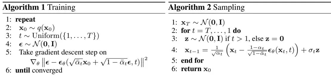
Algorithm 1 Training; Algorithm 2 Sampling

💡 Training & Sampling:

Training

2. $\mathbf{x}_0\sim q(\mathbf{x}_0)$ ：从训练集采样一张干净图像 $x_0$。这里的 $q(x_0)$ 是真实数据的经验分布，不是前向加噪转移。

3. $t\sim\mathrm{Uniform}(\{1,\ldots,T\})$ ：从全部扩散时间步中均匀抽取一个 $t$，每个样本只负责训练一个随机噪声等级，长期训练后所有时间步都会被覆盖。

4. $\boldsymbol\epsilon\sim\mathcal N(\mathbf{0},\mathbf I)$ ：采样一个与 $x_0$ 同形状的标准高斯噪声 $\epsilon$，用来构造训练输入 $x_t$，并作为网络需要预测的监督标签。

5. 计算损失并更新 $\theta$ ：

5.1 构造带噪输入：用式 (4) 一步得到时刻 $t$ 的图像：

$$\mathbf{x}_t=\sqrt{\bar\alpha_t}\mathbf{x}_0+\sqrt{1-\bar\alpha_t}\boldsymbol\epsilon.$$

5.2 预测噪声：把 $x_t$ 和时间步 $t$ 输入网络：

$$\hat{\boldsymbol\epsilon} = \boldsymbol\epsilon_\theta(\mathbf{x}_t,t).$$

5.3 计算损失：比较真实噪声与预测噪声，得到后文式 (14) 的均方误差：

$$\ell = \left\| \boldsymbol\epsilon-\hat{\boldsymbol\epsilon} \right\|^2.$$

5.4 更新参数：反向传播 $\nabla_\theta\ell$，由优化器更新网络参数 $\theta$。$\alpha_t$、$\bar\alpha_t$ 和本次采样的 $\epsilon$ 都不参与学习。

Sampling

1. $\mathbf{x}_T\sim\mathcal N(\mathbf{0},\mathbf I)$ ：从标准高斯分布采样初始噪声 $x_T$，最终图像将从这个随机张量逐步形成。

2. $t=T,\ldots,1$ ：从 $T$ 到 $1$ 依次执行反向过程：

3. $\mathbf z\sim\mathcal N(\mathbf{0},\mathbf I)$ if $t>1$, else $\mathbf z=\mathbf 0$ ：当 $t>1$ 时，采样一个与 $x_t$ 同形状的新噪声 $z$，用来保留反向过程的随机性；当 $t=1$ 时令 $z=0$，避免对最终结果再次添加噪声。

4. 由 $x_t$ 计算 $x_{t-1}$ ：

4.1 预测噪声：把当前状态 $x_t$ 和时间步 $t$ 输入训练好的网络：

$$\hat{\boldsymbol\epsilon} = \boldsymbol\epsilon_\theta(\mathbf{x}_t,t).$$

4.2 计算反向均值：从 $x_t$ 中减去网络预测的噪声分量，再补偿前向过程对信号的缩放：

$$\boldsymbol\mu_\theta(\mathbf{x}_t,t) = \frac1{\sqrt{\alpha_t}} \left( \mathbf{x}_t - \frac{1-\alpha_t}{\sqrt{1-\bar\alpha_t}} \hat{\boldsymbol\epsilon} \right).$$

其中，$1-\alpha_t=\beta_t$；中间的减法负责撤销当前噪声尺度下的一部分噪声，外面的 $1/\sqrt{\alpha_t}$ 负责还原前向一步造成的信号缩放。

4.3 完成一步采样：在反向均值附近加入方差为 $\sigma_t^2$ 的随机扰动：

$$\mathbf{x}_{t-1} = \boldsymbol\mu_\theta(\mathbf{x}_t,t) + \sigma_t\mathbf z.$$

当 $t=1$ 时 $z=0$，所以最后一步只保留反向均值，不再加入随机扰动。

最终生成图像 $x_0$

To summarize, we can train the reverse process mean function approximator $\boldsymbol{\mu}_\theta$ to predict $\tilde{\boldsymbol{\mu}}_t$, or by modifying its parameterization, we can train it to predict $\boldsymbol{\epsilon}$. (There is also the possibility of predicting $\mathbf{x}_0$, but we found this to lead to worse sample quality early in our experiments.) We have shown that the $\boldsymbol{\epsilon}$-prediction parameterization both resembles Langevin dynamics and simplifies the diffusion model’s variational bound to an objective that resembles denoising score matching. Nonetheless, it is just another parameterization of $p_\theta(\mathbf{x}_{t-1}\mid\mathbf{x}_t)$, so we verify its effectiveness in Section 4 in an ablation where we compare predicting $\boldsymbol{\epsilon}$ against predicting $\tilde{\boldsymbol{\mu}}_t$.

🧭 3.2 小结：

反向过程建模的是

$$p_\theta(\mathbf x_{t-1}\mid\mathbf x_t) = \mathcal N(\boldsymbol\mu_\theta,\sigma_t^2\mathbf I).$$

原始 DDPM 将方差 $\sigma_t^2$ 固定，因此核心只剩下如何表示均值 $\mu_\theta$。网络可以直接预测后验均值 $\tilde\mu_t$，也可以预测 $x_0$ 或噪声 $\epsilon$；它们本质上都是同一个反向高斯的不同参数化。

DDPM 最终采用 $\epsilon$-prediction：

$$\mathbf x_t \xrightarrow{\text{U-Net}} \boldsymbol\epsilon_\theta \xrightarrow{\text{式 (11)}} \boldsymbol\mu_\theta \xrightarrow{+\sigma_t\mathbf z} \mathbf x_{t-1}.$$

这种参数化把每个变分项化成式 (12) 的带时间权重噪声 MSE，并与 Denoising Score Matching 建立联系；第 3.4 节再去掉时间权重，得到 $L_{\mathrm{simple}}$。对应的随机反向采样则呈现出 Langevin-like 的形式。

3.3 Data scaling, reverse process decoder, and $L_0$

We assume that image data consists of integers in $\{0,1,\ldots,255\}$ scaled linearly to $[-1,1]$. This ensures that the neural network reverse process operates on consistently scaled inputs starting from the standard normal prior $p(\mathbf{x}_T)$. To obtain discrete log likelihoods, we set the last term of the reverse process to an independent discrete decoder derived from the Gaussian $\mathcal{N}(\mathbf{x}_0;\boldsymbol{\mu}_\theta(\mathbf{x}_1,1),\sigma_1^2\mathbf{I})$:

💡 式 (13)｜连续高斯如何给离散像素概率:

模型最后输出的是连续高斯，但真实图片是 256 个离散像素值，所以必须把连续密度转换成合法的离散概率：

原始像素整数 $k\in\{0,\ldots,255\}$ 被映射到 $[-1,1]$ ，则有：

$$x=\frac{2k}{255}-1.$$

相邻两个离散值在 $[-1,1]$ 上相距 $2/255$，因此每个内部像素值对应一个半宽为 $1/255$ 的量化区间：

$$\left[ x-\frac1{255}, x+\frac1{255} \right].$$

第一步：计算一个坐标的概率质量。

对第 $i$ 个像素通道，最后一步网络给出连续高斯

$$\mathcal N\!\left( x; \mu_\theta^i(\mathbf{x}_1,1), \sigma_1^2 \right).$$

记其均值为 $\mu_i$，标准差为 $\sigma_1$，则离散值 $x_0^i$ 的概率不是高斯在一个点上的密度，而是对应区间中的积分：

$$P_i = \int_{\delta_-(x_0^i)}^{\delta_+(x_0^i)} \mathcal N(x;\mu_i,\sigma_1^2)\,dx.$$

实现时可用标准高斯 CDF $\Phi$ 计算：

$$P_i = \Phi\!\left( \frac{\delta_+(x_0^i)-\mu_i}{\sigma_1} \right) - \Phi\!\left( \frac{\delta_-(x_0^i)-\mu_i}{\sigma_1} \right).$$

第二步：处理边界值。

对 $x_0^i=-1$，下界设为 $-\infty$；对 $x_0^i=1$，上界设为 $+\infty$。这样高斯落在有效像素范围之外的尾部概率也归入最靠近的边界值，全部 256 个离散 bin 的概率和仍为 1。

第三步：组合整张图像。

解码器假设给定 $x_1$ 后各坐标条件独立，所以

$$p_\theta(\mathbf{x}_0\mid\mathbf{x}_1) = \prod_{i=1}^{D}P_i, \qquad L_0 = -\sum_{i=1}^{D}\log P_i.$$

其中 $D=HWC$。这使模型得到的是合法的离散图像概率质量，从而可以把 $L_0$ 和整个变分界解释为无损码长。

where $D$ is the data dimensionality and the $i$ superscript indicates extraction of one coordinate. (It would be straightforward to instead incorporate a more powerful decoder like a conditional autoregressive model, but we leave that to future work.) Similar to the discretized continuous distributions used in VAE decoders and autoregressive models [34, 52], our choice here ensures that the variational bound is a lossless codelength of discrete data, without need of adding noise to the data or incorporating the Jacobian of the scaling operation into the log likelihood. At the end of sampling, we display $\boldsymbol{\mu}_\theta(\mathbf{x}_1,1)$ noiselessly.

⚙️ 实现含义: 计算 L0 或评估 likelihood 时，需要稳定计算两个相近 CDF 的差，边界位置则直接使用单侧 CDF。生成时，输出最后一步均值 $\mu_\theta(\mathbf{x}_1,1)$，不再采样加噪。本文假设给定 x1 后不同像素坐标条件独立，计算简单，但无法描述它们之间残留的相关性；更强的自回归解码器可以放宽这一假设，代价是更复杂、更慢，本文不考虑。

3.4 Simplified training objective

With the reverse process and decoder defined above, the variational bound, consisting of terms derived from Eqs. (12) and (13), is clearly differentiable with respect to $\theta$ and is ready to be employed for training. However, we found it beneficial to sample quality (and simpler to implement) to train on the following variant of the variational bound:

$$L_{\mathrm{simple}}(\theta) := \mathbb{E}_{t,\mathbf{x}_0,\boldsymbol{\epsilon}} \!\left[ \left\| \boldsymbol{\epsilon} -\boldsymbol{\epsilon}_\theta\!\left( \sqrt{\bar{\alpha}_t}\mathbf{x}_0 +\sqrt{1-\bar{\alpha}_t}\boldsymbol{\epsilon}, t \right) \right\|^2 \right]. \tag{14}$$

where $t$ is uniform between $1$ and $T$. The $t=1$ case corresponds to $L_0$ with the integral in the discrete decoder definition (13) approximated by the Gaussian probability density function times the bin width, ignoring $\sigma_1^2$ and edge effects. The $t>1$ cases correspond to an unweighted version of Eq. (12), analogous to the loss weighting used by the NCSN denoising score matching model [55]. ($L_T$ does not appear because the forward process variances $\beta_t$ are fixed.) Algorithm 1 displays the complete training procedure with this simplified objective.

Since our simplified objective (14) discards the weighting in Eq. (12), it is a weighted variational bound that emphasizes different aspects of reconstruction compared to the standard variational bound [18, 22]. In particular, our diffusion process setup in Section 4 causes the simplified objective to down-weight loss terms corresponding to small $t$. These terms train the network to denoise data with very small amounts of noise, so it is beneficial to down-weight them so that the network can focus on more difficult denoising tasks at larger $t$ terms. We will see in our experiments that this reweighting leads to better sample quality.

💡 式 (14)｜从严格 ELBO 到简化噪声 MSE:

前面由 ELBO 推导得到，对于 $t>1$，单步损失可以写成带权的噪声预测误差：

$$L_{t-1} = \mathbb E \left[ w_t \left\| \boldsymbol\epsilon- \boldsymbol\epsilon_\theta(\mathbf x_t,t) \right\|^2 \right] +C,$$

其中

$$w_t = \frac{\beta_t^2} {2\sigma_t^2\alpha_t(1-\bar\alpha_t)}.$$

也就是说，严格按照 ELBO 训练时，不同时间步的噪声预测误差具有不同的重要性。

原始 DDPM 发现，直接去掉这个时间权重效果反而更好，于是定义

$$L_{\mathrm{simple}} = \mathbb E_{t,\mathbf x_0,\boldsymbol\epsilon} \left[ \left\| \boldsymbol\epsilon- \boldsymbol\epsilon_\theta(\mathbf x_t,t) \right\|^2 \right],$$

其中

$$\mathbf x_t = \sqrt{\bar\alpha_t}\mathbf x_0 + \sqrt{1-\bar\alpha_t}\boldsymbol\epsilon, \qquad t\sim\mathrm{Uniform}\{1,\ldots,T\}.$$

在本文采用的噪声日程下，原来的 $w_t$ 相对强调较小的 $t$。这些时刻噪声很少，$x_t$ 已经非常接近原图，去噪任务较容易。去掉 $w_t$ 后，相当于降低低噪声重建的相对重要性，让网络投入更多能力处理较大 $t$ 下更困难的去噪任务，实验中因此获得了更好的生成质量。

$t=1$ 原本对应离散 decoder 的

$$L_0=-\log p_\theta(\mathbf x_0\mid\mathbf x_1),$$

作者用“高斯密度 $\times$ bin 宽度”近似式 (13) 的积分，使其也可以统一到噪声预测目标中；$L_T$ 则因为噪声日程 $\beta_t$ 固定、对 $\theta$ 没有梯度而直接忽略。

因此，$L_{\mathrm{simple}}$ 不再严格等于原始 ELBO，而是对不同时间步重新加权后的训练目标。它更偏向生成质量而非精确 likelihood：实验中这种重加权改善了 sample quality，但会牺牲一部分 likelihood。

最终训练流程:

$$\mathbf x_0 \xrightarrow[\epsilon\sim\mathcal N(0,I)]{\text{随机选择 }t} \mathbf x_t \xrightarrow{\epsilon_\theta(\mathbf x_t,t)} \hat{\boldsymbol\epsilon} \xrightarrow{\mathrm{MSE}} \left\|\boldsymbol\epsilon-\hat{\boldsymbol\epsilon}\right\|^2.$$

🔖 Section 总结

第 3 节把 DDPM 从概率定义落到可执行算法：固定前向日程与反向方差后，逐步高斯 KL 化成均值误差；解析代换又表明预测后验均值可等价参数化为预测噪声。式 (11) 把 $\epsilon_\theta$ 转成反向均值，式 (12) 将它保留在变分目标中，式 (14) 则通过去掉时间权重换取更好的样本质量。离散解码器负责把最后一步连续高斯转成合法像素概率，而训练一步与采样千步之间的计算不对称构成原始 DDPM 的主要效率代价。

核心洞察

1. $\epsilon$ prediction 是反向均值 $\mu_\theta$ 的一种参数化。
2. 固定 $\Sigma_\theta=\sigma_t^2I$ 让每个 KL 变成加权 MSE；简单稳定的代价是无法学习样本相关的反向不确定性。
3. 训练可随机抽一个 $t$ 并一步构造 $x_t$，采样却必须从 $T$ 到 $1$ 串行运行同一网络。
4. $L_{\mathrm{simple}}$ 改变了时间步权重，因此可以改善 FID（数值降低），同时牺牲一部分 likelihood / lossless codelength。
5. $L_0$ 的离散 bin 积分使变分界能够按离散图像的无损码长解释。

4 Experiments

📌 预览

本节检验 DDPM 的样本质量、反向参数化消融、渐进编码和潜空间插值，并记录实现成本与评测口径。阅读时优先区分训练集/测试集 FID、原始 ELBO/$L_{\mathrm{simple}}$ 与“概念性压缩/可部署压缩”，避免把不同口径的数字或机制解释混为一谈。

4 Experiments

We set $T=1000$ for all experiments so that the number of neural network evaluations needed during sampling matches previous work [53, 55]. We set the forward process variances to constants increasing linearly from $\beta_1=10^{-4}$ to $\beta_T=0.02$. These constants were chosen to be small relative to data scaled to $[-1,1]$, ensuring that reverse and forward processes have approximately the same functional form while keeping the signal-to-noise ratio at $\mathbf{x}_T$ as small as possible ($L_T=D_{\mathrm{KL}}(q(\mathbf{x}_T\mid\mathbf{x}_0)\parallel\mathcal{N}(\mathbf{0},\mathbf{I}))\approx10^{-5}$ bits per dimension in our experiments).

To represent the reverse process, we use a U-Net backbone similar to an unmasked PixelCNN++ [52, 48] with group normalization throughout [66]. Parameters are shared across time, which is specified to the network using the Transformer sinusoidal position embedding [60]. We use self-attention at the $16\times16$ feature map resolution [63, 60]. Details are in Appendix B.

💡 实验主设置:

• 扩散步数：所有实验固定 $T=1000$。一次训练更新只抽取一个时间步，但生成一张图必须串行调用网络 1000 次；这里选择 1000 主要是为了与此前工作保持相同的采样预算，并不是对速度最优的结论。
• 噪声日程：$\beta_t$ 从 $10^{-4}$ 线性增加到 $0.02$。单步噪声相对 $[-1,1]$ 的图像尺度较小，使前向与反向转移都可用小步高斯近似；终点的 $L_T\approx10^{-5}$ bits/dim，说明 $q(x_T\mid x_0)$ 已非常接近标准高斯先验。
• 网络结构：所有时间步共享同一个 U-Net，通过正弦时间嵌入区分噪声强度。卷积负责局部建模，self-attention 只放在 $16\times16$ 特征层，用较低成本引入全局交互。

4.1 Sample quality

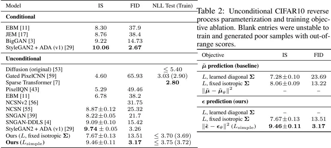
Table 1: CIFAR10 results. NLL measured in bits/dim. Table 2: Unconditional CIFAR10 reverse process parameterization and training objective ablation. Blank entries were unstable to train and generated poor samples with out-of-range scores.

💡 Table 1–2｜先统一指标方向:

• IS 越高越好，衡量生成图像能否同时做到类别明确且整体多样；它依赖 Inception 分类器，不能替代人工质量判断。
• FID 越低越好，比较真实图像与生成图像的特征分布；reference set 不同会改变数值，因此训练集 FID 3.17 与测试集 FID 5.24 必须分开报告。
• NLL / bits per dimension 越低越好，对应无损编码长度。表中的 $\leq$ 表明报告的是变分上界，而不是精确 NLL。

左侧 Table 1 的同模型对照最关键：固定方差的原始变分目标 $L$ 得到 FID 13.51、NLL $\leq3.70$；$L_{\mathrm{simple}}$ 得到 FID 3.17、NLL $\leq3.75$。去掉时间权重显著改善样本质量，却让码长略差，说明感知质量与 likelihood 并不完全同向。

右侧 Table 2 用来拆分参数化、目标函数和方差设置的作用，具体在第 4.2 节解读。空白格表示训练不稳定并产生超出正常范围的分数，不能按零值理解。

Table 1 shows Inception scores, FID scores, and negative log likelihoods (lossless codelengths) on CIFAR10. With our FID score of 3.17, our unconditional model achieves better sample quality than most models in the literature, including class conditional models. Our FID score is computed with respect to the training set, as is standard practice; when we compute it with respect to the test set, the score is 5.24, which is still better than many of the training set FID scores in the literature.

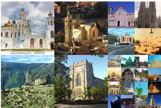
Figure 3: LSUN Church samples. FID=7.89

💡 图示解读: 样本能稳定生成教堂轮廓、尖顶和植被纹理，说明模型已学到场景的整体结构；但补充 Table 3 中 DDPM 的 FID 7.89 仍高于 StyleGAN2 的 3.86。左上样本还出现了明显的 Shutterstock 水印，说明模型也会复现训练数据中的水印与文字偏差；这反映数据分布中的伪特征，但不能仅凭一张图断言逐样本记忆。该图证明视觉样本具有合理性，却不能证明 DDPM 在 LSUN Church 上达到最佳结果。

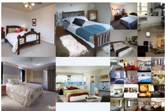
Figure 4: LSUN Bedroom samples. FID=4.90

💡 图示解读: 大模型能生成多种床铺位置、视角和室内布局；扩大模型后，Bedroom FID 从 6.36 降至 4.90，但仍高于 StyleGAN 的 2.65。左下样本同样带有水印片段，再次说明模型会学习数据集中的非语义伪影。图像展示适合检查结构与多样性，跨模型排序仍应以统一评测口径下的 FID 为准。

We find that training our models on the true variational bound yields better codelengths than training on the simplified objective, as expected, but the latter yields the best sample quality. See Fig. 1 for CIFAR10 and CelebA-HQ $256\times256$ samples, Fig. 3 and Fig. 4 for LSUN $256\times256$ samples [71], and Appendix D for more.

⚖️ 指标权衡: 原始变分界直接优化无损码长，因此 NLL 更好；$L_{\mathrm{simple}}$ 重新分配不同噪声尺度的训练权重，因此 FID/IS 更好。这里最有说服力的是同一模型家族内的目标消融，它支持“两个目标偏好不同”，但不能推出 likelihood 对所有生成任务都不重要。

4.2 Reverse process parameterization and training objective ablation

In Table 2, we show the sample quality effects of reverse process parameterizations and training objectives (Section 3.2). We find that the baseline option of predicting $\tilde{\boldsymbol{\mu}}_t$ works well only when trained on the true variational bound instead of unweighted mean squared error, a simplified objective akin to Eq. (14). We also see that learning reverse process variances (by incorporating a parameterized diagonal $\boldsymbol{\Sigma}_\theta(\mathbf{x}_t)$ into the variational bound) leads to unstable training and poorer sample quality compared to fixed variances. Predicting $\boldsymbol{\epsilon}$, as we proposed, performs approximately as well as predicting $\tilde{\boldsymbol{\mu}}_t$ when trained on the variational bound with fixed variances, but much better when trained with our simplified objective.

💡 Table 2｜消融如何定位有效组合:

预测目标	训练目标与方差	FID	结论
$\tilde\mu_t$	原始 $L$，学习对角方差	23.69	可训练，但质量最差
$\tilde\mu_t$	原始 $L$，固定各向同性方差	13.22	固定方差明显更稳定
$\tilde\mu_t$	无权均值 MSE	—	训练不稳定
$\epsilon$	原始 $L$，学习对角方差	—	训练不稳定
$\epsilon$	原始 $L$，固定各向同性方差	13.51	与 $\tilde\mu_t$ 的 13.22 接近
$\epsilon$	$L_{\mathrm{simple}}$，固定方差	3.17	最佳组合

这组对照说明，FID 的大幅改善不能只归因于“预测 $\epsilon$”：在同为原始 $L$、固定方差时，两种参数化几乎持平。真正有效的是 $\epsilon$ 参数化与时间步重加权的组合。学习对角方差的失败只适用于本文训练配方，不能推出“学习方差一般无效”。

4.3 Progressive coding

Table 1 also shows the codelengths of our CIFAR10 models. The gap between train and test is at most 0.03 bits per dimension, which is comparable to the gaps reported with other likelihood-based models and indicates that our diffusion model is not overfitting (see Appendix D for nearest neighbor visualizations). Still, while our lossless codelengths are better than the large estimates reported for energy based models and score matching using annealed importance sampling [11], they are not competitive with other types of likelihood-based generative models [7].

Since our samples are nonetheless of high quality, we conclude that diffusion models have an inductive bias that makes them excellent lossy compressors. Treating the variational bound terms $L_1+\cdots+L_T$ as rate and $L_0$ as distortion, our CIFAR10 model with the highest quality samples has a rate of 1.78 bits/dim and a distortion of 1.97 bits/dim, which amounts to a root mean squared error of 0.95 on a scale from 0 to 255. More than half of the lossless codelength describes imperceptible distortions.

💡 从无损码长拆出 rate 与 distortion:

对最佳样本模型，变分码长约为

$$\underbrace{1.78}_{L_1+\cdots+L_T\;\text{：传输潜变量}} + \underbrace{1.97}_{L_0\;\text{：补齐精确像素}} = 3.75\ \text{bits/dim}.$$

前面的 1.78 bits/dim 让接收端逐步获得足以重建图像的潜变量；最后的 $L_0$ 再把近似重建补成逐像素完全一致的无损结果。此时近似重建的 RMSE 已只有 0.95（像素尺度为 $[0,255]$），但精确补齐仍消耗 1.97 bits/dim，超过总码长的一半。论文所谓“多数码长描述不可感知失真”，指的正是这部分对视觉影响很小、对无损恢复却必不可少的像素细节。

训练集与测试集码长相差不超过 0.03 bits/dim，说明该模型没有明显记忆训练集；但其绝对码长仍弱于强 likelihood 模型，因此“擅长有损表示”不能等同于“擅长无损压缩”。

Progressive lossy compression We can probe further into the rate-distortion behavior of our model by introducing a progressive lossy code that mirrors the form of Eq. (5): see Algorithms 3 and 4, which assume access to a procedure, such as minimal random coding [19, 20], that can transmit a sample $\mathbf{x}\sim q(\mathbf{x})$ using approximately $D_{\mathrm{KL}}(q(\mathbf{x})\parallel p(\mathbf{x}))$ bits on average for any distributions $p$ and $q$, for which only $p$ is available to the receiver beforehand. When applied to $\mathbf{x}_0\sim q(\mathbf{x}_0)$, Algorithms 3 and 4 transmit $\mathbf{x}_T,\ldots,\mathbf{x}_0$ in sequence using a total expected codelength equal to Eq. (5). The receiver, at any time $t$, has the partial information $\mathbf{x}_t$ fully available and can progressively estimate:

Algorithms 3–4: progressive transmission

Algorithm 3 Sending $\mathbf{x}_0$

1. Send $\mathbf{x}_T\sim q(\mathbf{x}_T\mid\mathbf{x}_0)$ using $p(\mathbf{x}_T)$.
2. For $t=T-1,\ldots,2,1$ do.
3. Send $\mathbf{x}_t\sim q(\mathbf{x}_t\mid\mathbf{x}_{t+1},\mathbf{x}_0)$ using $p_\theta(\mathbf{x}_t\mid\mathbf{x}_{t+1})$.
4. End for.
5. Send $\mathbf{x}_0$ using $p_\theta(\mathbf{x}_0\mid\mathbf{x}_1)$.

Algorithm 4 Receiving

1. Receive $\mathbf{x}_T$ using $p(\mathbf{x}_T)$.
2. For $t=T-1,\ldots,1,0$ do.
3. Receive $\mathbf{x}_t$ using $p_\theta(\mathbf{x}_t\mid\mathbf{x}_{t+1})$.
4. End for.
5. Return $\mathbf{x}_0$.

💡 Algorithms 3–4:

• 发送端知道原图 $x_0$：先从 $q(x_T\mid x_0)$ 选择终点 latent，再从真实前向后验 $q(x_t\mid x_{t+1},x_0)$ 依次选择 $x_{T-1},\ldots,x_1$，最后发送精确的 $x_0$。
• **“using $p$”**是把接收端已知的 $p(x_T)$ 或 $p_\theta(x_t\mid x_{t+1})$ 当作编码参考分布。样本实际来自 $q$，二者的不匹配决定需要额外发送多少信息。
• 接收端按照同样的参考分布解码，因此能依次恢复与发送端一致的中间状态。每收到一个 $x_t$，它就可以先形成一个当前精度的重建，不必等到完整无损码流结束。
• 在理想 minimal random coding 下，传输一次 $x\sim q$ 的平均代价约为 $D_{\mathrm{KL}}(q\parallel p)$；把所有时间步相加，恰好得到式 (5) 的各项。

这一解释依赖理想编码过程。附录明确指出 minimal random coding 对高维数据不可处理，因此 Algorithms 3–4 只说明 ELBO 可以解释为渐进码长，并不是可直接部署的压缩算法。

$$\mathbf{x}_0 \approx \hat{\mathbf{x}}_0 = \frac{ \mathbf{x}_t - \sqrt{1-\bar\alpha_t}\, \boldsymbol\epsilon_\theta(\mathbf{x}_t) }{ \sqrt{\bar\alpha_t} }. \tag{15}$$

💡 式 (15)｜收到 $x_t$ 后如何立即预览原图:

式 (4) 的采样形式为

$$\mathbf x_t = \sqrt{\bar\alpha_t}\mathbf x_0 + \sqrt{1-\bar\alpha_t}\boldsymbol\epsilon.$$

接收端不知道真实噪声 $\epsilon$，于是用网络预测 $\epsilon_\theta(x_t,t)$ 替换它，再反解 $x_0$：

$$\hat{\mathbf x}_0 = \frac{ \mathbf x_t-\sqrt{1-\bar\alpha_t}\,\boldsymbol\epsilon_\theta(\mathbf x_t,t) }{ \sqrt{\bar\alpha_t} }.$$

这是给定当前 $x_t$ 的确定性点估计，用它计算 RMSE 才能让不同时间步的 distortion 可直接比较。也可以从 $p_\theta(x_0\mid x_t)$ 随机采样重建，但额外随机性会让失真曲线更难解释。式 (15) 原文省略了网络输入中的时间步 $t$，实现时仍需要提供。

due to Eq. (4). (A stochastic reconstruction $\mathbf{x}_0\sim p_\theta(\mathbf{x}_0\mid\mathbf{x}_t)$ is also valid, but we do not consider it here because it makes distortion more difficult to evaluate.) Figure 5 shows the resulting rate-distortion plot on the CIFAR10 test set. At each time $t$, the distortion is calculated as the root mean squared error $\sqrt{\|\mathbf{x}_0-\hat{\mathbf{x}}_0\|^2/D}$, and the rate is calculated as the cumulative number of bits received so far at time $t$. The distortion decreases steeply in the low-rate region of the rate-distortion plot, indicating that the majority of the bits are indeed allocated to imperceptible distortions.

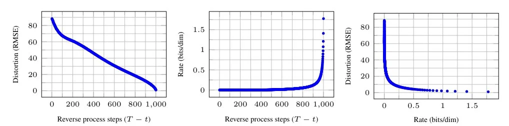
Figure 5: Unconditional CIFAR10 test set rate-distortion vs. time. Distortion is measured in root mean squared error on a [0, 255] scale. See Table 4 for details.

💡 Figure 5:

• 左图（步数–失真）：随着反向步数 $T-t$ 从 0 增至 1000，RMSE 从接近 90 降到 1 以下，说明重建信息沿反向链持续增加。
• 中图（步数–码率）：累计 rate 在大部分反向过程接近零，到最后一段才快速上升；越接近精确像素，新增信息越昂贵。
• 右图（码率–失真）：最初极少量 bit 就能大幅降低 RMSE，随后增加大量 bit 只换来较小的数值改进，这就是“先语义结构、后精细像素”的 rate–distortion 表现。

三图支持“多数无损码长花在感知不敏感细节”这一解释，但证据来自特定 CIFAR10 模型和 RMSE 失真度量；换数据集、感知指标或实际编码器，曲线不一定相同。

Progressive generation We also run a progressive unconditional generation process given by progressive decompression from random bits. In other words, we predict the result of the reverse process, $\hat{\mathbf{x}}_0$, while sampling from the reverse process using Algorithm 2. Figures 6 and 10 show the resulting sample quality of $\hat{\mathbf{x}}_0$ over the course of the reverse process. Large scale image features appear first and details appear last. Figure 7 shows stochastic predictions $\mathbf{x}_0\sim p_\theta(\mathbf{x}_0\mid\mathbf{x}_t)$ with $\mathbf{x}_t$ frozen for various $t$. When $t$ is small, all but fine details are preserved, and when $t$ is large, only large scale features are preserved. Perhaps these are hints of conceptual compression [18].

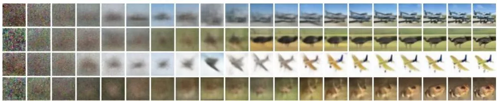
Figure 6: Unconditional CIFAR10 progressive generation ($\hat{\mathbf{x}}_0$ over time, from left to right). Extended samples and sample quality metrics over time in the appendix (Figs. 10 and 14).

💡 图示解读: 图中展示的是每个中间状态 $x_t$ 经式 (15) 得到的 $\hat x_0$，不是原始的带噪 $x_t$。从左到右，类别轮廓和大色块先稳定，局部纹理最后补齐；它把 Figure 5 的数值曲线转化为可见的 coarse-to-fine 生成过程。

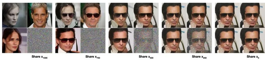
Figure 7: When conditioned on the same latent, CelebA-HQ $256 \times 256$ samples share high-level attributes. Bottom-right quadrants are $\mathbf{x}_t$, and other quadrants are samples from $p_\theta(\mathbf{x}_0\mid\mathbf{x}_t)$.

💡 图示解读: 每组右下角固定同一个 $x_t$，其余三个象限是从 $p_\theta(x_0\mid x_t)$ 独立继续采样的结果。$t$ 较大时，$x_t$ 只约束大尺度属性，不同分支可以形成不同身份和细节；$t$ 越小，共享信息越具体，最终在 $t=0$ 时退化为同一张图。这说明反向过程的随机性主要补全当前 latent 尚未确定的内容。

Connection to autoregressive decoding Note that the variational bound (5) can be rewritten as:

$$L = D_{\mathrm{KL}}\!\left( q(\mathbf{x}_T)\parallel p(\mathbf{x}_T) \right) + \mathbb E_q\!\left[ \sum_{t\geq1} D_{\mathrm{KL}}\!\left( q(\mathbf{x}_{t-1}\mid\mathbf{x}_t) \parallel p_\theta(\mathbf{x}_{t-1}\mid\mathbf{x}_t) \right) \right] + H(\mathbf{x}_0). \tag{16}$$

💡 式 (16)｜把变分界改写成“模型误差 + 数据熵”:

• 第一项比较终点边缘分布 $q(x_T)$ 与先验 $p(x_T)$；噪声日程足够长时，这一项接近零。
• 中间各项比较真实反向条件分布 $q(x_{t-1}\mid x_t)$ 与模型 $p_\theta(x_{t-1}\mid x_t)$；它们衡量每个反向步骤还没有学到的部分。
• $H(x_0)$ 是真实数据本身不可消除的熵，与模型参数无关。

因此，如果先验和所有反向条件分布都拟合完美，前两部分都降到零，剩下的最低码长就是数据熵 $H(x_0)$。这个写法也为下面的自回归思想实验提供了入口。

(See Appendix A for a derivation.) Now consider setting the diffusion process length $T$ to the dimensionality of the data, defining the forward process so that $q(\mathbf{x}_t\mid\mathbf{x}_0)$ places all probability mass on $\mathbf{x}_0$ with the first $t$ coordinates masked out (i.e. $q(\mathbf{x}_t\mid\mathbf{x}_{t-1})$ masks out the $t^{\mathrm{th}}$ coordinate), setting $p(\mathbf{x}_T)$ to place all mass on a blank image, and, for the sake of argument, taking $p_\theta(\mathbf{x}_{t-1}\mid\mathbf{x}_t)$ to be a fully expressive conditional distribution. With these choices, $D_{\mathrm{KL}}(q(\mathbf{x}_T)\parallel p(\mathbf{x}_T))=0$, and minimizing $D_{\mathrm{KL}}(q(\mathbf{x}_{t-1}\mid\mathbf{x}_t)\parallel p_\theta(\mathbf{x}_{t-1}\mid\mathbf{x}_t))$ trains $p_\theta$ to copy coordinates $t+1,\ldots,T$ unchanged and to predict the $t^{\mathrm{th}}$ coordinate given $t+1,\ldots,T$. Thus, training $p_\theta$ with this particular diffusion is training an autoregressive model.

We can therefore interpret the Gaussian diffusion model (2) as a kind of autoregressive model with a generalized bit ordering that cannot be expressed by reordering data coordinates. Prior work has shown that such reorderings introduce inductive biases that have an impact on sample quality [38], so we speculate that the Gaussian diffusion serves a similar purpose, perhaps to greater effect since Gaussian noise might be more natural to add to images compared to masking noise. Moreover, the Gaussian diffusion length is not restricted to equal the data dimension; for instance, we use $T=1000$, which is less than the dimension of the $32\times32\times3$ or $256\times256\times3$ images in our experiments. Gaussian diffusions can be made shorter for fast sampling or longer for model expressiveness.

💡 为什么这能视作广义自回归: 这个思想实验把“加噪”特化为按坐标逐个遮盖：前向第 $t$ 步遮掉第 $t$ 个坐标，反向第 $t$ 步便根据尚未遮挡的 $t+1,\ldots,T$ 预测第 $t$ 个坐标，同时复制其余已知坐标。这恰好得到一个固定顺序的自回归分解。

高斯扩散并不逐个遮掉像素，而是在每个噪声尺度同时更新所有坐标，所以它的“顺序”沿信噪比展开，无法表示成简单的像素排列。作者将其解释为一种可能有利于图像的归纳偏置，但没有证明这种 Gaussian bit ordering 必然最优。链长 $T$ 仍需在采样速度与单步建模难度之间权衡。

🧭 4.3 小结: 同一条变分链可以从三种角度理解：训练时，它分解负对数似然上界；在理想通信协议中，它逐步传输 latent 并形成 rate–distortion 曲线；把高斯加噪替换成逐坐标 masking 时，它又退化为普通自回归解码。后两者是对数学结构的解释或特殊构造，本文真正训练的仍是高斯扩散模型；minimal random coding 也仍不可扩展到高维实用压缩。

4.4 Interpolation

We can interpolate source images $\mathbf{x}_0,\mathbf{x}'_0\sim q(\mathbf{x}_0)$ in latent space using $q$ as a stochastic encoder, $\mathbf{x}_t,\mathbf{x}'_t\sim q(\mathbf{x}_t\mid\mathbf{x}_0)$, then decoding the linearly interpolated latent $\bar{\mathbf{x}}_t=(1-\lambda)\mathbf{x}_0+\lambda\mathbf{x}'_0$ into image space by the reverse process, $\bar{\mathbf{x}}_0\sim p(\mathbf{x}_0\mid\bar{\mathbf{x}}_t)$. In effect, we use the reverse process to remove artifacts from linearly interpolating corrupted versions of the source images, as depicted in Fig. 8 (left). We fixed the noise for different values of $\lambda$ so $\mathbf{x}_t$ and $\mathbf{x}'_t$ remain the same. Fig. 8 (right) shows interpolations and reconstructions of original CelebA-HQ $256\times256$ images ($t=500$). The reverse process produces high-quality reconstructions, and plausible interpolations that smoothly vary attributes such as pose, skin tone, hairstyle, expression and background, but not eyewear. Larger $t$ results in coarser and more varied interpolations, with novel samples at $t=1000$ (Appendix Fig. 9).

⚠️ 原文公式的下标笔误: 本段先用前向过程把两张源图随机编码到同一噪声层级：

$$\mathbf{x}_t\sim q(\mathbf{x}_t\mid\mathbf{x}_0), \qquad \mathbf{x}'_t\sim q(\mathbf{x}'_t\mid\mathbf{x}'_0).$$

因此线性插值的对象应当是两个带噪 latent，而不是两张干净源图：

$$\bar{\mathbf{x}}_t =(1-\lambda)\mathbf{x}_t+\lambda\mathbf{x}'_t.$$

随后从时间步 $t$ 开始运行反向扩散，将插值后的 latent 解码回图像：

$$\bar{\mathbf{x}}_0 \sim p_\theta(\mathbf{x}_0\mid\bar{\mathbf{x}}_t).$$

如果沿用 PDF 中的 $\mathbf{x}_0,\mathbf{x}'_0$，前一句构造的 $\mathbf{x}_t,\mathbf{x}'_t$ 就完全没有被使用，$\bar{\mathbf{x}}_t$ 也不再位于时间步 $t$ 的带噪空间。Figure 8 和官方实现都采用修正后的流程。

原文的 “fixed the noise” 是说改变 $\lambda$ 时固定已经采样出的两个带噪端点，避免端点重新采样干扰插值比较；它不表示两张源图必须共用同一份噪声。官方代码分别生成两个端点，并保留了是否改用共享噪声的 TODO。

Figure 8: Interpolations of CelebA-HQ 256x256 images with 500 timesteps of diffusion.

💡 Figure 8｜插值粒度由 $t$ 控制: 左图对比了直接在像素空间连线与“先加噪、在 latent 中连线、再去噪”的路径；反向模型把容易产生重影和模糊的线性混合拉回到学到的图像流形附近。右图中姿态、肤色、发型、表情和背景大体连续变化，但眼镜没有平滑过渡，说明该空间能表达部分连续语义，却没有让所有属性都解耦；单组可视化也不足以证明整个潜空间都具有线性语义。

较小的 $t$ 保留更多源图信息，插值主要改变局部外观；较大的 $t$ 破坏更多细节，反向过程拥有更大的重建自由度，因此结果更粗粒度、更多样。当 $t=1000$ 时，源图信息几乎消失，插值结果更接近新生成的样本，而不是两张原图的精细混合。

Extra information

LSUN FID scores for LSUN datasets are included in Table 3. Scores marked with ∗ are reported by StyleGAN2 as baselines, and other scores are reported by their respective authors.

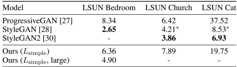
Table 3: FID scores for LSUN 256 × 256 datasets

💡 Table 3: 标准 DDPM 在 Bedroom、Church、Cat 上的 FID 分别为 6.36、7.89、19.75；扩大模型只报告了 Bedroom，并将其改善到 4.90，但仍高于 StyleGAN 的 2.65。Church 和 Cat 也落后于表中最佳基线，说明 CIFAR10 上的优势不能直接外推到所有 LSUN 类别。

Progressive compression Our lossy compression argument in Section 4.3 is only a proof of concept, because Algorithms 3 and 4 depend on a procedure such as minimal random coding [20], which is not tractable for high dimensional data. These algorithms serve as a compression interpretation of the variational bound (5) of Sohl-Dickstein et al. [53], not yet as a practical compression system.

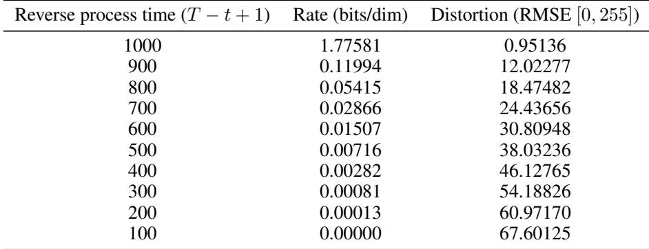
Table 4: Unconditional CIFAR10 test set rate-distortion values (accompanies Fig. 5)

💡 Table 4｜Figure 5 的精确数值: 从 100 到 1000 个反向步骤，累计 rate 从近 0 增至 1.77581 bits/dim，RMSE 从 67.60125 降至 0.95136。前 900 步只累计约 0.12 bits/dim，最后 100 步却增加约 1.66 bits/dim；这定量说明多数码长集中在反向末段。至于这些比特对应何种视觉内容，需要结合 Figure 6 的渐进图像判断，不能只由 RMSE 表格推出。

🔖 Section 总结

实验首先验证了 $\epsilon$ prediction 与 $L_{\mathrm{simple}}$ 的组合能够显著改善 CIFAR10 样本质量，但 NLL 略差，说明 likelihood 与感知质量并不完全同向。消融表明收益来自参数化、目标重加权和固定方差的共同配合，而不是单独更换预测目标。渐进编码实验进一步显示反向链先确定大尺度结构、后补像素细节，但其压缩解释仍依赖不可扩展的理想编码过程；LSUN 结果也表明该方法并未在所有数据类别上领先。

关键数字

证据	关键数字	应如何解读
CIFAR10 最佳样本质量	IS 9.46；训练集 FID 3.17；测试集 FID 5.24	3.17 使用训练集作 FID reference，跨论文比较必须核对口径
目标函数权衡	原始 $L$：FID 13.51、NLL $\leq3.70$；$L_{\mathrm{simple}}$：FID 3.17、NLL $\leq3.75$ bits/dim	重加权显著改善感知质量，但无损码长略差
原始采样成本	$T=1000$ 次串行网络求值	训练可抽单个 $t$，生成成本却随 $T$ 线性增长
渐进编码端点	rate 1.77581 bits/dim；distortion 1.97 bits/dim；RMSE 0.95136	总变分码长约 3.75 bits/dim；大部分 rate 在反向末段累积，且只对应概念性编码
LSUN FID	Bedroom 4.90（large）；Church 7.89；Cat 19.75	结果对类别和模型容量敏感，并非所有 LSUN 类别都领先

核心洞察

1. 最佳 CIFAR10 结果来自 $\epsilon$ prediction 与 $L_{\mathrm{simple}}$ 的组合，不能归因于噪声参数化本身。
2. 在本文训练配方下，固定反向方差比学习对角方差更稳定；这一结论不代表学习方差一般无效。
3. FID 的改善伴随 NLL 略差，说明生成质量与无损似然需要分别评估。
4. $T=1000$ 次串行网络求值是原始 DDPM 的主要推理瓶颈。
5. 渐进压缩与广义自回归是对变分链的机制解释，不是本文已经实现的高维实用压缩器。

5 Related Work and Appendix C

📌 预览

本节简要定位 DDPM 与 VAE、flow、score-based model 等路线的关系。Appendix C 的重点是：DDPM 的训练目标与实际 sampler 由同一前向过程共同推导。

5 Related Work

While diffusion models might resemble flows [9, 46, 10, 32, 5, 16, 23] and VAEs [33, 47, 37], diffusion models are designed so that $q$ has no parameters and the top-level latent $\mathbf{x}_T$ has nearly zero mutual information with the data $\mathbf{x}_0$. Our $\boldsymbol{\epsilon}$-prediction reverse process parameterization establishes a connection between diffusion models and denoising score matching over multiple noise levels with annealed Langevin dynamics for sampling [55, 56]. Diffusion models, however, admit straightforward log likelihood evaluation, and the training procedure explicitly trains the Langevin dynamics sampler using variational inference (see Appendix C for details). The connection also has the reverse implication that a certain weighted form of denoising score matching is the same as variational inference to train a Langevin-like sampler. Other methods for learning transition operators of Markov chains include infusion training [2], variational walkback [15], generative stochastic networks [1], and others [50, 54, 36, 42, 35, 65].

By the known connection between score matching and energy-based modeling, our work could have implications for other recent work on energy-based models [67–69, 12, 70, 13, 11, 41, 17, 8]. Our rate-distortion curves are computed over time in one evaluation of the variational bound, reminiscent of how rate-distortion curves can be computed over distortion penalties in one run of annealed importance sampling [24]. Our progressive decoding argument can be seen in convolutional DRAW and related models [18, 40] and may also lead to more general designs for subscale orderings or sampling strategies for autoregressive models [38, 64].

💡 DDPM 的交叉定位:

在本文的高斯参数化下，带权 denoising score matching 可以写成有限步变分目标。VAE、flow 和 DRAW 主要提供模型家族或结构类比；与自回归模型的等价则只在特殊的 masking diffusion 下成立。原文所谓 likelihood evaluation 指计算变分上界，并非精确边缘似然。

C Discussion on related work

Our model architecture, forward process definition, and prior differ from NCSN [55, 56] in subtle but important ways that improve sample quality, and, notably, we directly train our sampler as a latent variable model rather than adding it after training post-hoc. In greater detail:

1. We use a U-Net with self-attention; NCSN uses a RefineNet with dilated convolutions. We condition all layers on $t$ by adding in the Transformer sinusoidal position embedding, rather than only in normalization layers (NCSNv1) or only at the output (v2).

2. Diffusion models scale down the data with each forward process step (by a $\sqrt{1-\beta_t}$ factor) so that variance does not grow when adding noise, thus providing consistently scaled inputs to the neural net reverse process. NCSN omits this scaling factor.

3. Unlike NCSN, our forward process destroys signal ($D_{\mathrm{KL}}(q(\mathbf{x}_T\mid\mathbf{x}_0)\parallel\mathcal{N}(\mathbf{0},\mathbf{I}))\approx0$), ensuring a close match between the prior and aggregate posterior of $\mathbf{x}_T$. Also unlike NCSN, our $\beta_t$ are very small, which ensures that the forward process is reversible by a Markov chain with conditional Gaussians. Both of these factors prevent distribution shift when sampling.

4. Our Langevin-like sampler has coefficients (learning rate, noise scale, etc.) derived rigorously from $\beta_t$ in the forward process. Thus, our training procedure directly trains our sampler to match the data distribution after $T$ steps: it trains the sampler as a latent variable model using variational inference. In contrast, NCSN’s sampler coefficients are set by hand post-hoc, and their training procedure is not guaranteed to directly optimize a quality metric of their sampler.

💡 DDPM 与 NCSN 的核心区别: DDPM 用同一组 $\beta_t$ 定义前向加噪，并进一步推导 ELBO、反向均值和采样系数；本文所比较的 NCSN 则先学习多噪声尺度 score，再配置 annealed Langevin sampler。因此，“directly trains the sampler” 指训练目标包含实际执行的有限步反向转移。Appendix C 同时改变了架构、缩放和 sampler 等多项设计，不能据此判断每一项的独立贡献。

🔖 Section 总结

DDPM 最关键的定位是：$\epsilon$ prediction 既能参数化反向均值，也对应多噪声尺度 score 学习；固定前向链又把这一目标与有限步 sampler 连接起来。

核心洞察

1. 带权 denoising score matching 与本文的有限步变分目标直接相关。
2. DDPM 的前向过程、训练目标和 sampler 由同一组 $\beta_t$ 串联起来。
3. Appendix C 是多项设计的整体比较，不是逐因素消融。

6 Conclusion and Broader Impact

📌 预览

本节总结 DDPM 的贡献，并讨论生成伪造、数据偏差和潜在应用。

6 Conclusion

We have presented high quality image samples using diffusion models, and we have found connections among diffusion models and variational inference for training Markov chains, denoising score matching and annealed Langevin dynamics (and energy-based models by extension), autoregressive models, and progressive lossy compression. Since diffusion models seem to have excellent inductive biases for image data, we look forward to investigating their utility in other data modalities and as components in other types of generative models and machine learning systems.

💡 结论的证据边界: 论文已经在所测图像数据集上验证生成质量，并推导了 diffusion 与 score/Langevin、自回归分解和渐进编码的联系；其他模态、表征学习和系统集成仍是未来方向。扩散模型的建模方式天然比较符合图像的结构特点，因此容易学出视觉质量较好的结果。

Broader Impact

Our work on diffusion models takes on a similar scope as existing work on other types of deep generative models, such as efforts to improve the sample quality of GANs, flows, autoregressive models, and so forth. Our paper represents progress in making diffusion models a generally useful tool in this family of techniques, so it may serve to amplify any impacts that generative models have had (and will have) on the broader world.

Unfortunately, there are numerous well-known malicious uses of generative models. Sample generation techniques can be employed to produce fake images and videos of high profile figures for political purposes. While fake images were manually created long before software tools were available, generative models such as ours make the process easier. Fortunately, CNN-generated images currently have subtle flaws that allow detection [62], but improvements in generative models may make this more difficult. Generative models also reflect the biases in the datasets on which they are trained. As many large datasets are collected from the internet by automated systems, it can be difficult to remove these biases, especially when the images are unlabeled. If samples from generative models trained on these datasets proliferate throughout the internet, then these biases will only be reinforced further.

On the other hand, diffusion models may be useful for data compression, which, as data becomes higher resolution and as global internet traffic increases, might be crucial to ensure accessibility of the internet to wide audiences. Our work might contribute to representation learning on unlabeled raw data for a large range of downstream tasks, from image classification to reinforcement learning, and diffusion models might also become viable for creative uses in art, photography, and music.

⚠️ 影响:

• 更强的生成能力会降低伪造门槛；模型还可能复现互联网数据偏差，生成内容重新进入数据源后形成偏差反馈。
• 压缩有 rate–distortion 分析，但尚无可行编码器；表征学习、创意工具和其他模态均未在本文验证。

🔖 Section 总结

原始 DDPM 的贡献是展示高质量图像生成，并建立 diffusion、变分推断与 score/Langevin 等方法之间的联系。Broader Impact 只提出可能的收益与风险，没有进行实证评估。

核心洞察

1. 已验证贡献集中在图像生成和方法间的数学联系。
2. 其他模态、表征学习和实用压缩仍是设想，而非本文结果。
3. 能力提升可能同时放大伪造、数据偏差等风险与潜在用途。

Appendix A — Extended derivations

📌 预览

本节给出 ELBO 的两种分解。

A Extended derivations

Below is a derivation of Eq. (5), the reduced variance variational bound for diffusion models. This material is from Sohl-Dickstein et al. [53]; we include it here only for completeness.

$$L = \mathbb {E} _ {q} \biggl [ - \log \frac {p _ {\theta} (\mathbf {x} _ {0 : T})}{q (\mathbf {x} _ {1 : T} | \mathbf {x} _ {0})} \biggr ]\tag{17}$$

$$= \mathbb {E} _ {q} \left[ - \log p (\mathbf {x} _ {T}) - \sum_ {t \geq 1} \log \frac {p _ {\theta} (\mathbf {x} _ {t - 1} | \mathbf {x} _ {t})}{q (\mathbf {x} _ {t} | \mathbf {x} _ {t - 1})} \right]\tag{18}$$

$$= \mathbb {E} _ {q} \Bigg [ - \log p (\mathbf {x} _ {T}) - \sum_ {t > 1} \log \frac {p _ {\theta} (\mathbf {x} _ {t - 1} | \mathbf {x} _ {t})}{q (\mathbf {x} _ {t} | \mathbf {x} _ {t - 1})} - \log \frac {p _ {\theta} (\mathbf {x} _ {0} | \mathbf {x} _ {1})}{q (\mathbf {x} _ {1} | \mathbf {x} _ {0})} \Bigg ]\tag{19}$$

$$= \mathbb {E} _ {q} \Biggl [ - \log p (\mathbf {x} _ {T}) - \sum_ {t > 1} \log \frac {p _ {\theta} (\mathbf {x} _ {t - 1} | \mathbf {x} _ {t})}{q (\mathbf {x} _ {t - 1} | \mathbf {x} _ {t} , \mathbf {x} _ {0})} \cdot \frac {q (\mathbf {x} _ {t - 1} | \mathbf {x} _ {0})}{q (\mathbf {x} _ {t} | \mathbf {x} _ {0})} - \log \frac {p _ {\theta} (\mathbf {x} _ {0} | \mathbf {x} _ {1})}{q (\mathbf {x} _ {1} | \mathbf {x} _ {0})} \Biggr ]\tag{20}$$

$$= \mathbb {E} _ {q} \Biggl [ - \log \frac {p (\mathbf {x} _ {T})}{q (\mathbf {x} _ {T} | \mathbf {x} _ {0})} - \sum_ {t > 1} \log \frac {p _ {\theta} (\mathbf {x} _ {t - 1} | \mathbf {x} _ {t})}{q (\mathbf {x} _ {t - 1} | \mathbf {x} _ {t} , \mathbf {x} _ {0})} - \log p _ {\theta} (\mathbf {x} _ {0} | \mathbf {x} _ {1}) \Biggr ]\tag{21}$$

$$= \mathbb {E} _ {q} \Biggl [ D _ {\mathrm{KL}} (q (\mathbf {x} _ {T} | \mathbf {x} _ {0}) \parallel p (\mathbf {x} _ {T})) + \sum_ {t > 1} D _ {\mathrm{KL}} (q (\mathbf {x} _ {t - 1} | \mathbf {x} _ {t}, \mathbf {x} _ {0}) \parallel p _ {\theta} (\mathbf {x} _ {t - 1} | \mathbf {x} _ {t})) - \log p _ {\theta} (\mathbf {x} _ {0} | \mathbf {x} _ {1}) \Biggr ]\tag{22}$$

推导笔记见 02 Background：式 (3) → 式 (5)；三个分量如何进入模型训练，分别见 03.1：$L_T$、03.2：$L_{1:T-1}$ 和 03.3：$L_0$。

The following is an alternate version of $L$. It is not tractable to estimate, but it is useful for our discussion in Section 4.3.

$$L = \mathbb {E} _ {q} \Bigg [ - \log p (\mathbf {x} _ {T}) - \sum_ {t \geq 1} \log \frac {p _ {\theta} (\mathbf {x} _ {t - 1} | \mathbf {x} _ {t})}{q (\mathbf {x} _ {t} | \mathbf {x} _ {t - 1})} \Bigg ]\tag{23}$$

$$= \mathbb {E} _ {q} \Bigg [ - \log p (\mathbf {x} _ {T}) - \sum_ {t \geq 1} \log \frac {p _ {\theta} (\mathbf {x} _ {t - 1} | \mathbf {x} _ {t})}{q (\mathbf {x} _ {t - 1} | \mathbf {x} _ {t})} \cdot \frac {q (\mathbf {x} _ {t - 1})}{q (\mathbf {x} _ {t})} \Bigg ]\tag{24}$$

$$= \mathbb {E} _ {q} \left[ - \log \frac {p (\mathbf {x} _ {T})}{q (\mathbf {x} _ {T})} - \sum_ {t \geq 1} \log \frac {p _ {\theta} (\mathbf {x} _ {t - 1} | \mathbf {x} _ {t})}{q (\mathbf {x} _ {t - 1} | \mathbf {x} _ {t})} - \log q (\mathbf {x} _ {0}) \right]\tag{25}$$

$$= D _ {\mathrm{KL}} (q (\mathbf {x} _ {T}) \parallel p (\mathbf {x} _ {T})) + \mathbb {E} _ {q} \left[ \sum_ {t \geq 1} D _ {\mathrm{KL}} (q (\mathbf {x} _ {t - 1} | \mathbf {x} _ {t}) \parallel p _ {\theta} (\mathbf {x} _ {t - 1} | \mathbf {x} _ {t})) \right] + H (\mathbf {x} _ {0})\tag{26}$$

💡 式 (23)–(26)｜用于渐进编码解释:

1. 换用边缘 Bayes 公式：式 (24) 将前向转移写成 $q(x_{t-1}\mid x_t)q(x_t)/q(x_{t-1})$，不再条件于某个已知的 $x_0$。
2. 消去相邻边缘概率：连乘中的 $q(x_t)/q(x_{t-1})$ 消去，式 (25) 只留下终点比值、逐步反向比值与 $-\log q(x_0)$。
3. 识别信息量：取期望后，三部分分别成为终点先验 KL、各步反向条件 KL 和数据熵 $H(x_0)$，因此每一步 KL 可以解释为渐进编码所需的额外 rate。

🔖 Section 总结

附录 A 的第一套分解对应正文使用的可训练 ELBO；第二套分解改用真实边缘逆条件，将目标写成数据熵与逐步额外码率，主要服务于渐进编码解释。

Appendix B — Experimental details

📌 预览

本节记录复现原始 DDPM 所需的网络、噪声日程、优化器、训练成本和评测口径。重点区分经过比较的选择、未经 sweep 的固定值，以及从 CIFAR10 直接迁移到其他数据集的设置。

B Experimental details

Our neural network architecture follows the backbone of PixelCNN++ [52], which is a U-Net [48] based on a Wide ResNet [72]. We replaced weight normalization [49] with group normalization [66] to make the implementation simpler. Our $32\times32$ models use four feature map resolutions ($32\times32$ to $4\times4$), and our $256\times256$ models use six. All models have two convolutional residual blocks per resolution level and self-attention blocks at the $16\times16$ resolution between the convolutional blocks [6]. Diffusion time $t$ is specified by adding the Transformer sinusoidal position embedding [60] into each residual block. Our CIFAR10 model has 35.7 million parameters, and our LSUN and CelebA-HQ models have 114 million parameters. We also trained a larger variant of the LSUN Bedroom model with approximately 256 million parameters by increasing filter count.

💡 架构要点: 网络是带时间条件的多尺度 U-Net：32²/256² 模型分别使用 4/6 个分辨率，在 $16\times16$ 加 self-attention，并把正弦时间嵌入注入每个残差块。参数量从 CIFAR10 的 35.7M 增至基础高分辨率模型的 114M；大 Bedroom 模型约 256M。

We used TPU v3-8 (similar to 8 V100 GPUs) for all experiments. Our CIFAR model trains at 21 steps per second at batch size 128 (10.6 hours to train to completion at 800k steps), and sampling a batch of 256 images takes 17 seconds. Our CelebA-HQ/LSUN ($256^2$) models train at 2.2 steps per second at batch size 64, and sampling a batch of 128 images takes 300 seconds. We trained on CelebA-HQ for 0.5M steps, LSUN Bedroom for 2.4M steps, LSUN Cat for 1.8M steps, and LSUN Church for 1.2M steps. The larger LSUN Bedroom model was trained for 1.15M steps.

💡 成本口径:

设置	训练吞吐 / 时长	一批采样时间	说明
CIFAR10，$32^2$，35.7M	21 steps/s；800k steps ≈ 10.6 h	256 张 / 17 s	每张样本仍执行 1000 个反向步骤，只是 batch 并行
CelebA-HQ / LSUN，$256^2$，114M	2.2 steps/s	128 张 / 300 s	分辨率、尺度数和通道容量都更大

Apart from an initial choice of hyperparameters early on to make network size fit within memory constraints, we performed the majority of our hyperparameter search to optimize for CIFAR10 sample quality, then transferred the resulting settings over to the other datasets:

• We chose the $\beta_t$ schedule from a set of constant, linear, and quadratic schedules, all constrained so that $L_T\approx0$. We set $T=1000$ without a sweep, and we chose a linear schedule from $\beta_1=10^{-4}$ to $\beta_T=0.02$.

• We set the dropout rate on CIFAR10 to 0.1 by sweeping over the values 0.1, 0.2, 0.3, 0.4. Without dropout on CIFAR10, we obtained poorer samples reminiscent of the overfitting artifacts in an unregularized PixelCNN++ [52]. We set dropout rate on the other datasets to zero without sweeping.

• We used random horizontal flips during training for CIFAR10; we tried training both with and without flips, and found flips to improve sample quality slightly. We also used random horizontal flips for all other datasets except LSUN Bedroom.

• We tried Adam [31] and RMSProp early on in our experimentation process and chose the former. We left the hyperparameters to their standard values. We set the learning rate to $2\times10^{-4}$ without any sweeping, and we lowered it to $2\times10^{-5}$ for the $256\times256$ images, which seemed unstable to train with the larger learning rate.

• We set the batch size to 128 for CIFAR10 and 64 for larger images. We did not sweep over these values.

• We used EMA on model parameters with a decay factor of 0.9999. We did not sweep over this value.

💡 配置总结: 作者主要以 CIFAR10 样本质量为目标选择超参数，再将大部分设置迁移到其他数据集。最终采用线性噪声日程、$T=1000$、Adam、固定学习率与 batch size，并对模型参数使用 EMA。

Final experiments were trained once and evaluated throughout training for sample quality. Sample quality scores and log likelihood are reported on the minimum FID value over the course of training. On CIFAR10, we calculated Inception and FID scores on 50000 samples using the original code from the OpenAI [51] and TTUR [21] repositories, respectively. On LSUN, we calculated FID scores on 50000 samples using code from the StyleGAN2 [30] repository. CIFAR10 and CelebA-HQ were loaded as provided by TensorFlow Datasets (https://www.tensorflow.org/datasets), and LSUN was prepared using code from StyleGAN. Dataset splits (or lack thereof) are standard from the papers that introduced their usage in a generative modeling context. All details can be found in the source code release.

💡 评测总结: 每个最终实验只训练一次，并在训练过程中选择 FID 最低的 checkpoint 报告样本质量和 likelihood。CIFAR10 与 LSUN 均使用 50,000 个生成样本计算指标，并分别沿用对应的标准评测和数据准备代码。

🔖 Section 总结

Appendix B 给出了原始 DDPM 的完整复现配方，并量化了 1000 步采样的成本。解释结果时还必须保留搜索范围、跨数据集迁移和最低 FID checkpoint 选点等实验上下文。

关键数字

项目	数值
模型规模	CIFAR10：35.7M；高分辨率基础模型：114M；大 Bedroom：约 256M
CIFAR10 训练	batch 128；800k steps；约 10.6 h
采样时间	CIFAR10：256 张 / 17 s；256²：128 张 / 300 s
噪声日程	$T=1000$；线性 $\beta_1=10^{-4}\rightarrow\beta_T=0.02$
优化	Adam；LR $2\times10^{-4}$（256² 为 $2\times10^{-5}$）；EMA 0.9999
评测样本数	CIFAR10 / LSUN 均为 50,000

核心洞察

1. 同一 U-Net 通过时间嵌入覆盖全部噪声尺度，原始采样仍需串行执行 1000 步。
2. 多项关键超参数未经系统 sweep，且大部分设置从 CIFAR10 迁移到其他数据集。
3. 最佳 FID 来自单次训练中的 checkpoint 选点。

Appendix D — Samples

📌 预览

本节用未筛选样本、最近邻、渐进生成和插值补充主文指标。样本网格适合观察失败模式，最近邻只能排查简单复制，两者都不能单独证明分布覆盖或隐私安全。

D Samples

Additional samples Figure 11, 13, 16, 17, 18, and 19 show uncurated samples from the diffusion models trained on CelebA-HQ, CIFAR10 and LSUN datasets.

Latent structure and reverse process stochasticity During sampling, both the prior $\mathbf{x}_T\sim\mathcal{N}(\mathbf{0},\mathbf{I})$ and Langevin dynamics are stochastic. To understand the significance of the second source of noise, we sampled multiple images conditioned on the same intermediate latent for the CelebA $256\times256$ dataset. Figure 7 shows multiple draws from the reverse process $\mathbf{x}_0\sim p_\theta(\mathbf{x}_0\mid\mathbf{x}_t)$ that share the latent $\mathbf{x}_t$ for $t\in\{1000,750,500,250\}$. To accomplish this, we run a single reverse chain from an initial draw from the prior. At the intermediate timesteps, the chain is split to sample multiple images. When the chain is split after the prior draw at $\mathbf{x}_{T=1000}$, the samples differ significantly. However, when the chain is split after more steps, samples share high-level attributes like gender, hair color, eyewear, saturation, pose and facial expression. This indicates that intermediate latents like $\mathbf{x}_{750}$ encode these attributes, despite their imperceptibility.

💡 中间状态分叉: 多个样本先共享 $x_T$ 和一段反向轨迹，再从同一 $x_t$ 独立采样。$t$ 越小，分叉后的样本共享姿态、发色等属性越多，说明全局结构逐步固定；但“属性被编码”只是由输出相似性推断，并未训练属性解码器验证。

Coarse-to-fine interpolation Figure 9 shows interpolations between a pair of source CelebA $256\times256$ images as we vary the number of diffusion steps prior to latent space interpolation. Increasing the number of diffusion steps destroys more structure in the source images, which the model completes during the reverse process. This allows us to interpolate at both fine granularities and coarse granularities. In the limiting case of 0 diffusion steps, the interpolation mixes source images in pixel space. On the other hand, after 1000 diffusion steps, source information is lost and interpolations are novel samples.

插值与渐进生成

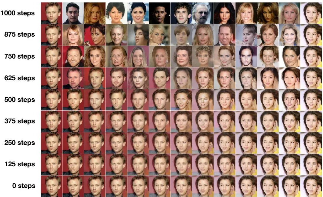
Figure 9: Coarse-to-fine interpolations that vary the number of diffusion steps prior to latent mixing.

💡 Figure 9: 列方向改变插值系数 $\lambda$，纵向改变混合前的加噪深度。$t=0$ 接近像素混合；$t$ 越大，源图约束越弱、模型补全越多，直至产生新样本。完整插值公式见 04 Experiments 的潜空间插值笔记

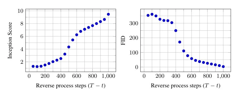
Figure 10: Unconditional CIFAR10 progressive sampling quality over time

💡 Figure 10: 横轴是已执行的反向步骤 $T-t$。IS 随采样推进上升、FID 下降，接近 1000 步才达到所报最终质量；这只说明直接截断原始链会损失质量，没有比较专门设计的少步 sampler。

未筛选样本与最近邻

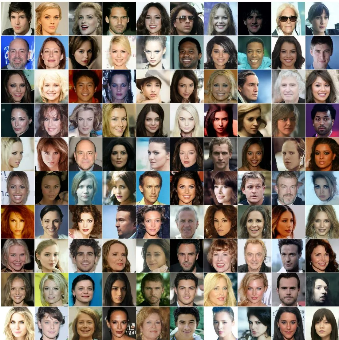
Figure 11: CelebA-HQ 256 × 256 generated samples

💡 Figure 11: 未筛选网格展示姿态、背景和发型的多样性，但不能估计长尾失败率、身份覆盖或训练数据记忆。

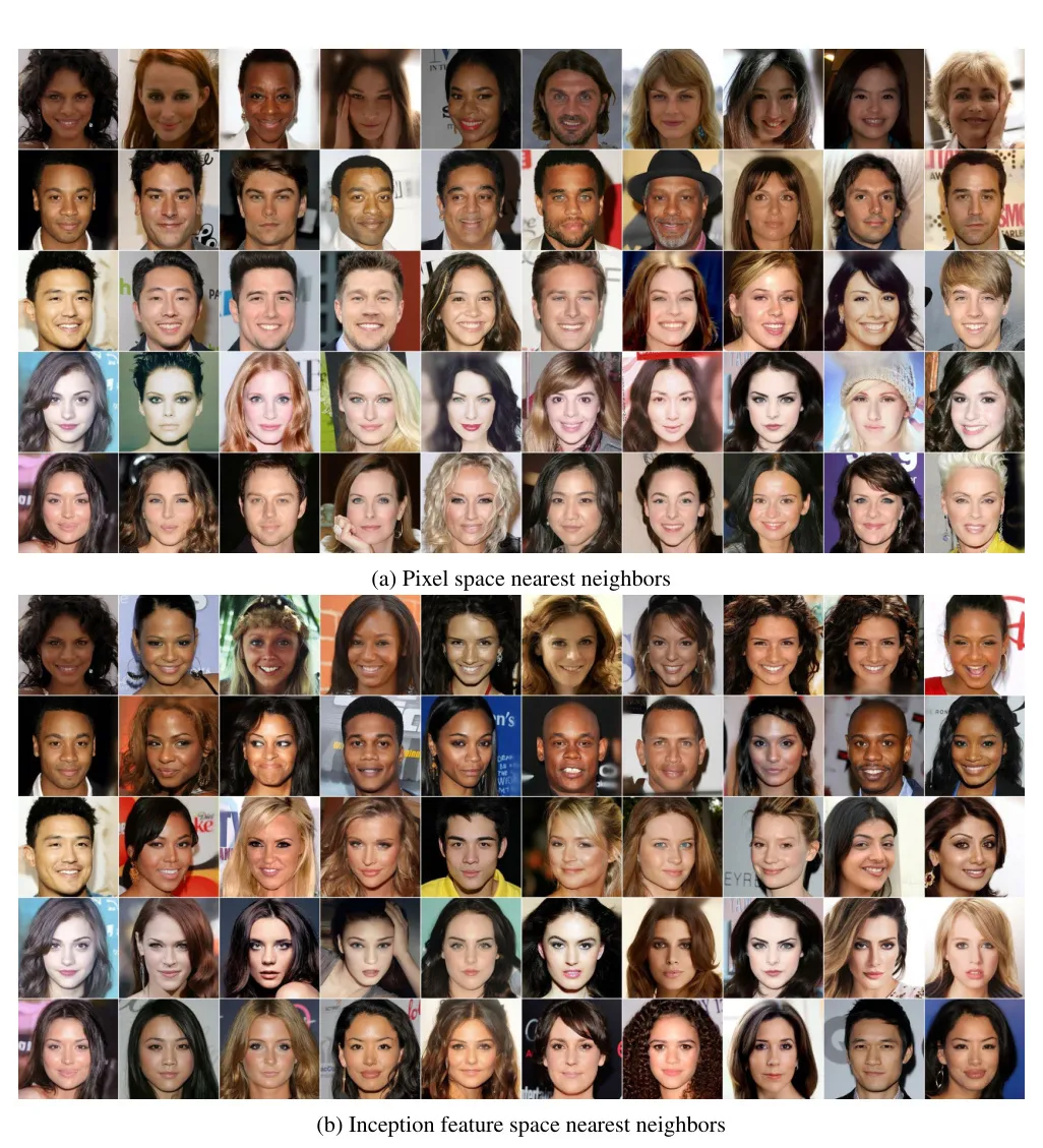
Figure 12: CelebA-HQ 256 × 256 nearest neighbors, computed on a 100 × 100 crop surrounding the faces. Generated samples are in the leftmost column, and training set nearest neighbors are in the remaining columns.

💡 Figure 12: 像素距离偏向颜色和位置对齐，Inception 特征更偏向语义外观。没有明显逐图复制只能排除最简单的记忆形式，不能排除组合复制或隐私泄漏。

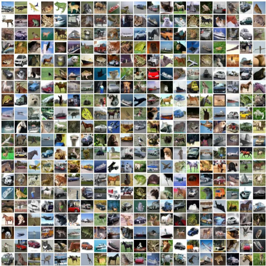
Figure 13: Unconditional CIFAR10 generated samples

💡 Figure 13: 无类别条件的模型生成了多种语义，但 $32\times32$ 分辨率限制了对纹理和局部伪影的判断。

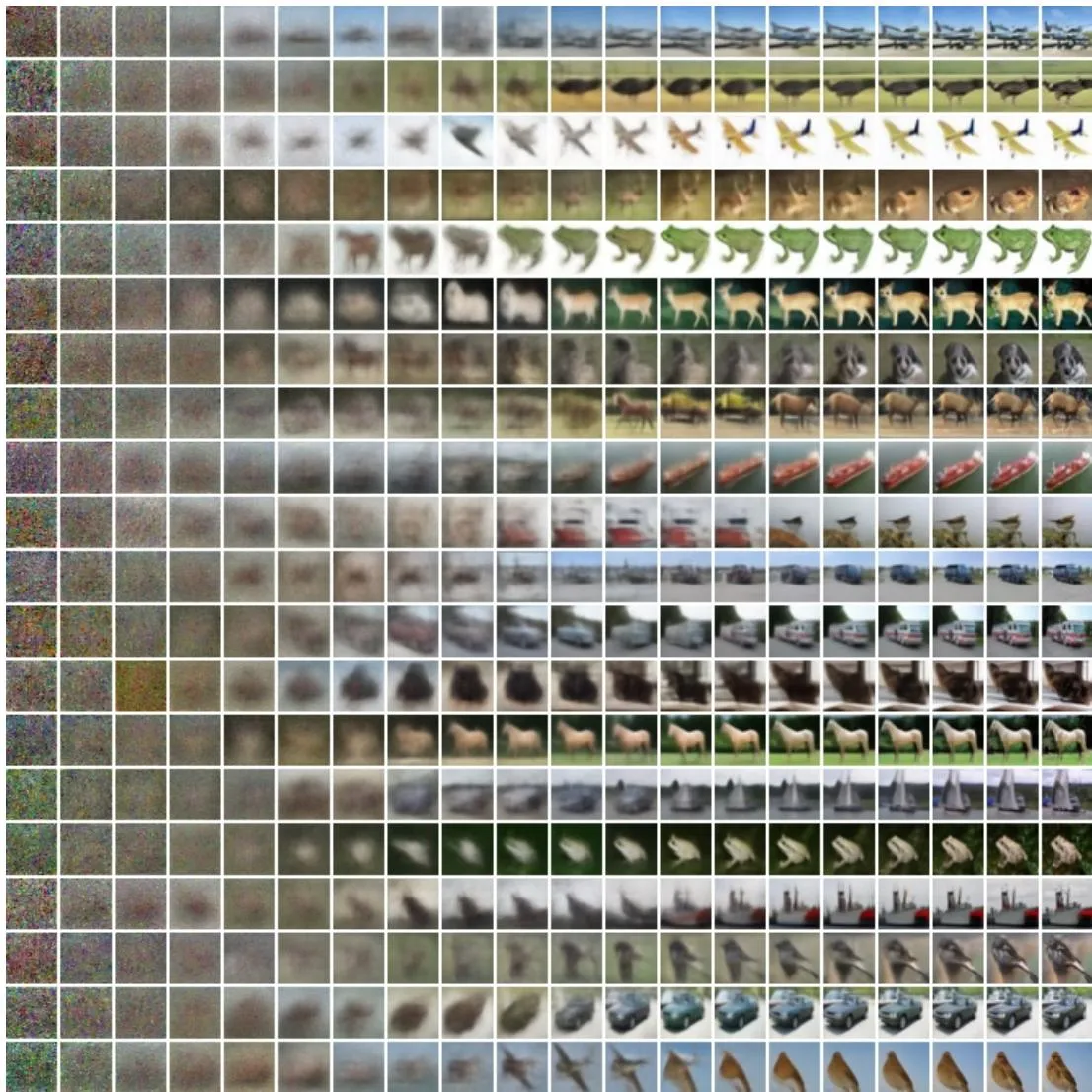
Figure 14: Unconditional CIFAR10 progressive generation

💡 Figure 14: 轨迹先形成大色块和类别轮廓，再细化边缘与纹理，与 04 Experiments 的渐进生成分析 一致。最终结果同时受初始 $x_T$ 和各步反向噪声影响，并非确定性解码。

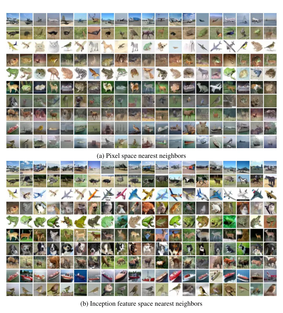
Figure 15: Unconditional CIFAR10 nearest neighbors. Generated samples are in the leftmost column, and training set nearest neighbors are in the remaining columns.

💡 Figure 15: 与 Figure 12 相同，两种距离只是在低层外观和语义相似性下排查最近邻；有限检索不能证明模型不存在 memorization。

LSUN 样本网格

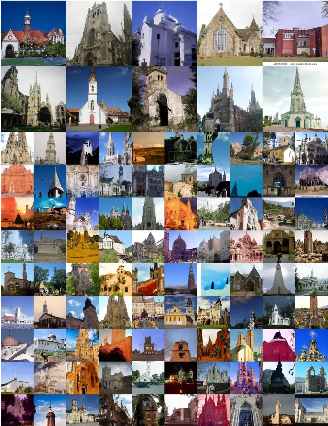
Figure 16: LSUN Church generated samples. FID=7.89

💡 Figure 16: Church 样本具有构图多样性，也出现几何失真和文字样伪影。FID 7.89 并非该类别的最佳结果，且不会直接揭示这些对象级失败。

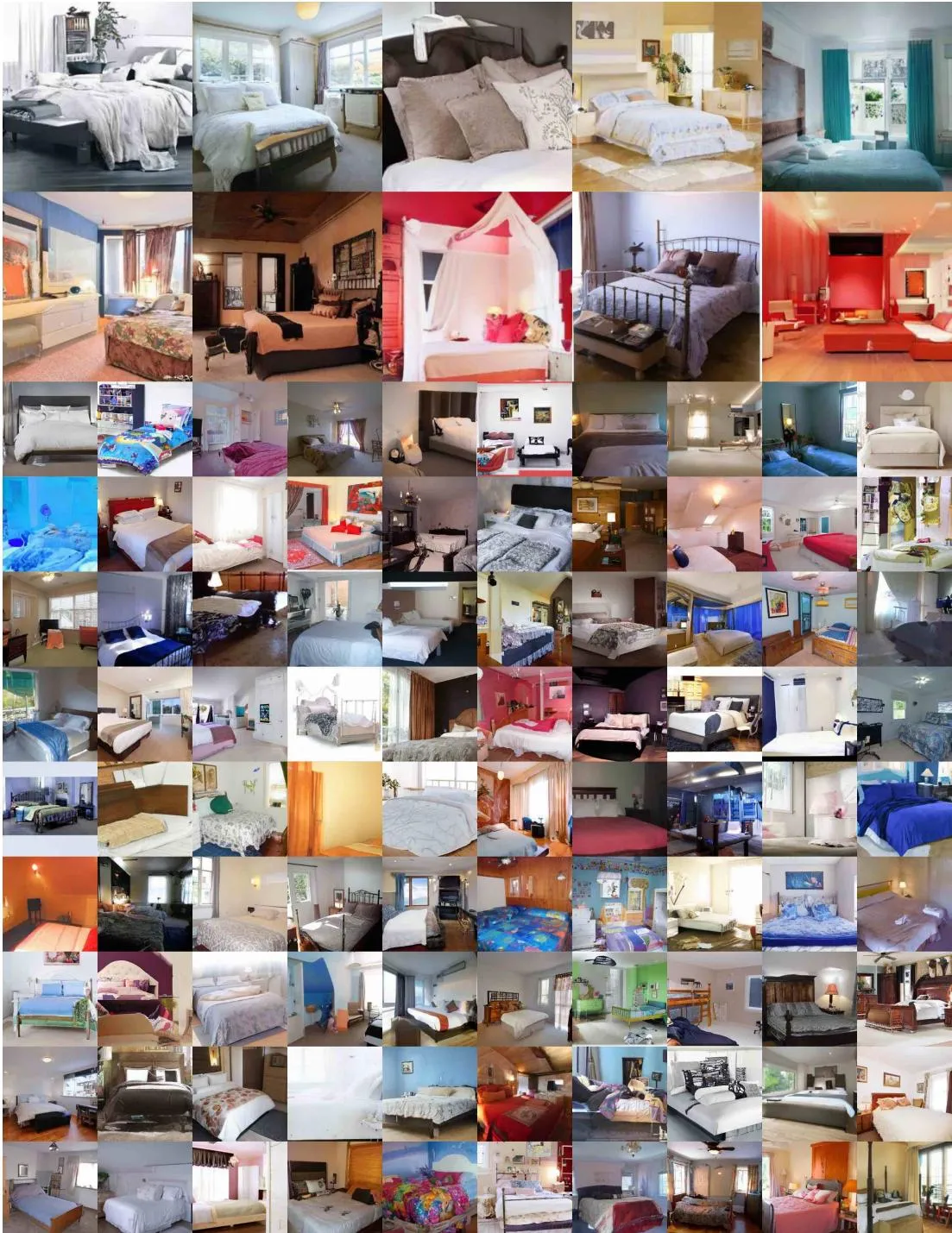
Figure 17: LSUN Bedroom generated samples, large model. FID=4.90

💡 Figure 17: 约 256M 参数的大模型得到 FID 4.90；与小模型比较时，模型容量和训练步数同时变化。

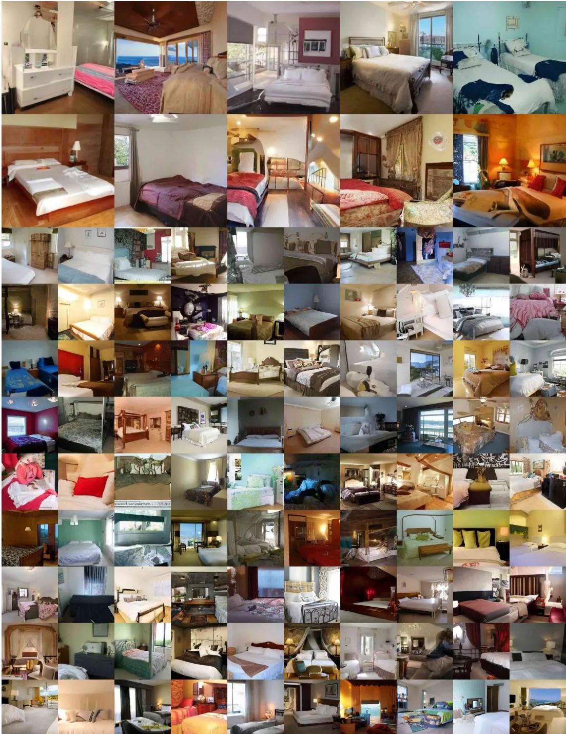
Figure 18: LSUN Bedroom generated samples, small model. FID=6.36

💡 Figure 18: 114M 小模型 FID 为 6.36，比大模型高 1.46；没有受控变量或重复运行，因此只能视为规模趋势。

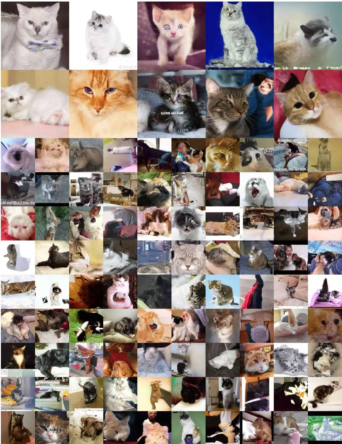
Figure 19: LSUN Cat generated samples. FID=19.75

💡 Figure 19: Cat 样本可见结构错乱、人与猫混合及文字样伪影；FID 19.75 是三个 LSUN 类别中最差的 DDPM 结果，说明 Bedroom 表现不能代表所有类别。

🔖 Section 总结

Appendix D 的视觉结果支持反向过程由粗到细的解释，并展示不同数据集上的常见成功与失败。中间状态分叉、最近邻和未筛选网格都只是诊断工具，不能替代覆盖率、隐私或因果表征评估。

关键数字

图 / 设置	数字	说明
中间 latent 分叉	$t\in\{1000,750,500,250\}$	$t$ 越小，共享属性越多
渐进质量	最终 IS 9.46 / FID 3.17	原始链需接近 1000 步才达到最终质量
LSUN FID	Bedroom 4.90/6.36；Church 7.89；Cat 19.75	类别差异显著，且 Bedroom 对比并非受控消融

核心洞察

1. 中间状态会逐步固定全局属性，反向链随后补充局部细节。
2. 最近邻和未筛选网格能发现简单问题，但不是完整的覆盖率或隐私审计。
3. LSUN 类别间差异明显，单一 Bedroom 结果不能代表整体能力。