基于生存分析的NIPT时间选择与胎儿异常判定
作者:余明羲,叶子枫,吴悠
摘要
无创产前检测(NIPT)因其高准确性和低风险在胎儿染色体异常筛查中得到广泛应用,但检测结果受孕周、BMI、胎儿性别等多因素影响。本文基于大规模孕妇检测数据,构建数学模型,系统分析了孕妇特征与胎儿性染色体浓度的关系,并提出数据驱动的BMI分组与最佳检测时点推荐方法。
对于问题一,本文首先对Y染色体浓度、孕期周数、BMI等数据进行了数据预处理和可视化分析,为后续模型的建立提供可靠的数据支持。随后,由于各变量均未通过 Sapiro–Wilk检验 ,使用Spearman偏相关系数 分析Y染色体浓度与孕妇各生理指标间的相关性。为验证并量化影响,进一步采用多元线性回归模型 ,用最小二乘法 拟合得到最终的模型,并进行残差分析以及显著性检验,计算得到决定系数**R 2 = 0.045 R^2=0.045 R 2 = 0.045 ,F统计量的p值为 1.66 × 10 − 8 1.66\times10^{-8} 1.66 × 1 0 − 8
对于问题二,本文采用结合 B样条 的半参数Cox比例风险模型 ,并为每个个体预测其95%成功率的达标孕周(Q95时间点)。由于临床数据删失严重,本文将每位孕妇的纵向观测数据转化为生存分析中的标准区间数据,并使用了多重插补(MI)缓解Cox比例风险模型无法处理的 左删失 问题。然后,本文利用保序回归 对此“BMI-Q95预测周数”关系进行单调化处理 ,以此为监督信号,通过回归树 算法寻找最优的BMI分组切点,得到4个分组,并结合剪枝与最小样本量等策略保证分组的稳健性。最后,在每个分组内,使用Kaplan–Meier 方法估计生存曲线和推荐检测时间点(t95),通过敏感性分析确认了模型在面对测量误差时的稳健性与可靠性。
对于问题三,为综合考虑多种因素对Y染色体浓度达标比例的影响,本文在问题二的生存分析框架下的标准区间数据的基础上,拟合包含BMI、年龄等协变量的区间删失 加速失效时间模型 (AFT),最佳分布为log-normal 。随后,本文对每个个体的首次达标时间分布进行初步估计,得到个体层的精确分布参数与分位点(Q90/Q95)及 π(25)=P(T≤25)。与问题二类似,为最大化组间差异,本文采用回归树 进行分组;在得到的3个分组内,采用基于 AFT 条件分布的多重插补(MI) ,再结合KM 方法估计生存曲线和推荐检测时间点(t95),当 KM 结果不可靠时则回退至 AFT 模型的组内中位预测。
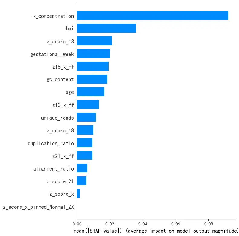
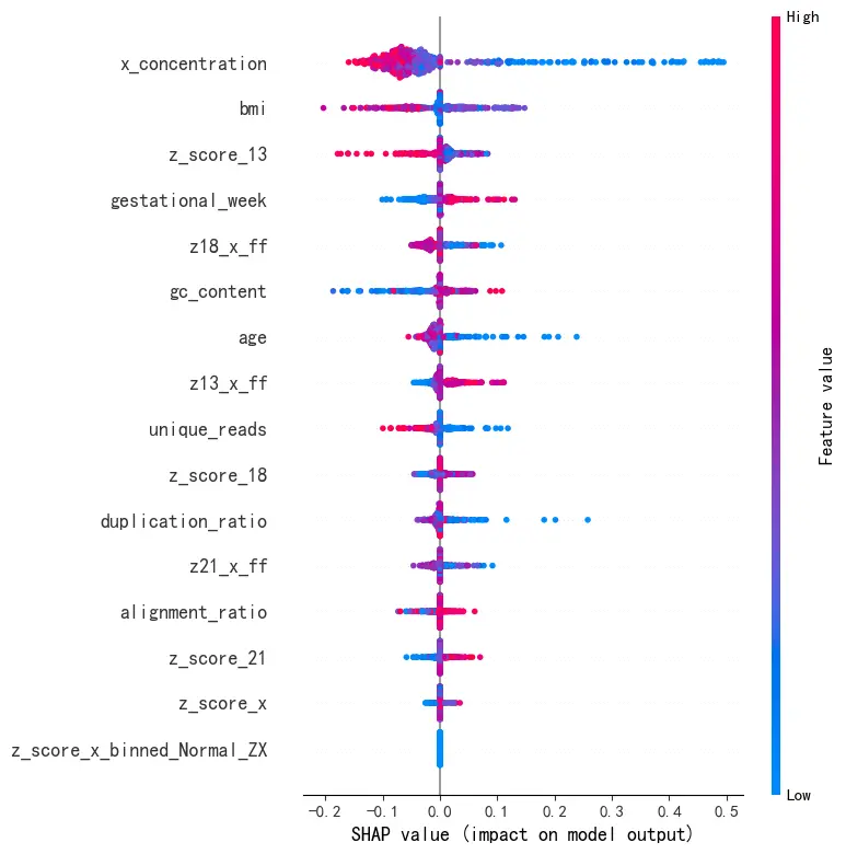
对于问题四,本文首先完成特征工程以增强原始数据。随后,考虑到临床上漏诊付出代价较高,本文以 最小化非对称临床代价函数 为唯一优化目标,构建了端到端集成学习模型 。该方法融合了XGBoost 和核SVM 两种模型的优势,并通过100次K折交叉验证 对所有超参数进行联合寻优。在验证集上,训练得到的最佳模型的临床代价为297 ,AUC 分数为 0.8216 ,表明模型具有良好的区分与预测能力。最后,本文使用SHAP 分析各特征的特征重要性并将结果可视化,增强了模型的可解释性及临床应用能力。
关键词: 多元线性回归, Cox模型, AFT模型, KM模型, 回归树, 集成学习模型
问题重述
问题背景
问题背景
尽管NIPT在临床中表现出较高的精确度,其结果仍受多种因素影响,尤其是胎儿性染色体浓度的测定——男胎的Y染色体或女胎的X染色体的游离DNA片段的测定比例。此外,不同孕妇的孕期、体重指数(BMI)以及胎儿的性别等因素都可能对检测结果产生影响。其中对于男胎,由于其携带Y染色体,其浓度的变化受到孕妇孕周数和BMI等因素的显著影响。
为了提高NIPT检测的准确性并降低潜在风险,临床实践中通常根据孕妇的BMI值对其进行分组,并根据不同群体的特点选择最佳的检测时点。然而,由于每个孕妇的个体差异,简单的经验分组并不能适用于所有情况。因此,如何在不同BMI组别中合理选择检测时点,确保检测准确性并尽量减少胎儿异常风险,是一个亟待解决的问题。
本研究旨在通过数学建模,分析胎儿性染色体浓度与孕妇的孕期、BMI等因素的关系,探讨如何根据不同孕妇群体的特点,优化NIPT的检测时点,以提高检测的准确性并降低早期发现异常所带来的潜在风险。同时,本文将考虑不同因素对检测误差的影响,以制定更加科学合理的分组策略和检测时点选择标准。
问题要求
本题以无创产前检测(NIPT)为背景,利用附件提供的孕妇检测数据,包括孕周、BMI、身高、体重、染色体浓度、Z值、GC含量等数据,用来研究胎儿染色体浓度的变化规律及其影响因素,建立数学模型,分析胎儿性染色体浓度与孕妇特征的关系,并确定不同孕妇群体的最佳检测时点,此外再针对女胎提出异常判定方法,旨在为临床优化NIPT检测策略提供科学依据。
问题1: 依据表格有关男胎的Y染色体浓度数据和孕妇特征数据,研究Y染色体浓度与孕周、BMI等变量的相关性,建立定量关系模型,并对模型进行显著性检验,验证关系是否可靠。
问题2: BMI是影响男胎Y染色体浓度最早达标时间的主要因素,需要按BMI对男胎孕妇进行分组并确定最佳检测时点(浓度首次大于等于4%),从而最小化潜在风险,并分析检测误差影响。
问题3: 在问题二中BMI分组的基础上,综合考虑身高、体重、年龄等多种因素,以及检测误差和达标比例(浓度达到或超过4%的比例),再结合男胎孕妇的BMI,适当调整分组情况以及每组的最佳NIPT时点,使得孕妇潜在风险达到最小化,并分析检测误差对结果的影响。
问题4: 针对女胎,为了明确女胎异常的判定方法,需结合21号、18号、13号染色体的Z值、GC含量、读段数及其比例、X染色体相关指标、孕妇BMI等特征,输出一个可用于判定女胎是否异常的模型或规则。
问题分析
问题一分析
针对问题一,本文选取孕妇的检测孕周、BMI、年龄三个指标,并对其与Y染色体浓度的偏相关性进行分析。首先通过Sapiro–Wilk检验 (W检验)确认了所有变量均不服从正态分布,因此本文选用非参数的Spearman偏相关性分析 替代 Pearson偏相关性分析,在控制其他变量后,即可得出Y染色体浓度与孕妇特征指标的偏相关性正负情况。其次,为验证并量化影响,进一步采用多元线性回归模型 ,并使用最小二乘法 来寻找最佳的系数估计值,由此得到最终的拟合模型。最后,对该回归模型进行评估,计算R 2 R^2 R 2
问题二分析
针对问题二,需要基于孕妇BMI对其分组,并为其推荐一个能以高概率成功检测到Y染色体的最优孕周。由于数据上严重的左删失 问题,本文将每位孕妇的纵向观测数据转化为生存分析框架 下的标准区间数据,明确标识出删失类型,并采用了多重插补(MI)技术,对删失区间内的真实达标时间进行合理的随机插补,以构建可供分析的完整数据集。然后,拟合结合 B样条 的半参数Cox比例风险模型 ,以灵活捕捉BMI对达标风险的非线性影响,并为每个个体预测其95%成功率的达标孕周(Q95时间点)。为确保业务逻辑的合理性,本文利用保序回归 对此“BMI-Q95预测周数”关系进行单调化处理 ,然后以此为监督信号,通过CART回归树 算法以数据驱动的方式寻找最优的BMI分组切点,并结合剪枝与最小样本量等策略保证分组的稳健性。最后,在每个分组内,使用Kaplan–Meier 方法估计生存曲线和推荐时间点(t95),再经跨组保序和半周圆整后得出最终推荐时点。为了分析检测误差对结果的影响,本文通过“模糊阈值”分析与“加噪蒙特卡洛 ”分析两种独立的敏感性分析来评估模型的稳健性,最终确认了模型在面对测量误差时的稳健性与可靠性。
问题三分析
针对问题三,需要在问题二的基础上考虑多种因素(如身高、体重、年龄等)的影响,对孕妇BMI对其进行分组,并为每组推荐一个最佳检测时点。在问题二的生存分析框架下的标准区间数据的基础上,首先拟合包含BMI、年龄等协变量的区间删失加速失效时间模型 (AFT),比较得出最佳分布为log-normal ,对每个个体的首次达标时间分布进行初步估计,得到个体层的精确分布参数与分位点(Q90/Q95)及 π(25)=P(T≤25)。其次,基于 AFT 模型的预测结果,利用CART回归树 以 π(25) 为监督信号(最小化SSE)进行分组,以最大化组间差异;在每个分组内,为在高删失背景下稳健估计组内生存曲线,采用基于 AFT 条件分布的多重插补(MI) ,再结合KM方法估计生存曲线和推荐时间点(t95),当 KM 结果不可靠时则回退至 AFT 模型的组内中位预测。此外,与问题二同理,本文通过“模糊区间”分析与“加噪蒙特卡洛 ”分析两种独立的敏感性分析来评估模型的稳健性,最终确认了模型在面对测量误差时的稳健性与可靠性。
问题四分析
针对女胎非整倍体异常的判定问题,核心挑战在于假阴性(漏诊)的临床代价远高于假阳性(误诊)。为应对此挑战,本文在进行特征工程 后,构建了一个以最小化非对称临床代价函数 为唯一优化目标的端到端集成学习模型 。该方法融合了XGBoost 和核SVM 两种模型的优势,并通过100次5折交叉验证对包括模型参数、集成权重和分类阈值在内的所有超参数进行联合寻优。此策略确保了最终模型的所有决策都精确地服务于“不惜代价降低漏诊率”这一核心临床需求,而非追求传统的准确率或AUC指标,从而在经过数据质控筛选后的高置信度样本上,实现了临床效用最大化的智能诊断。
符号说明
符号
说明
单位
$Y $
Y染色体浓度
/
$X_1 $
孕妇检测孕周
周
$X_2 $
孕妇BMI值
k g / m 2 kg/m^2 k g / m 2
$X_3 $
孕妇年龄
岁
$\beta $
回归系数
/
$\epsilon $
随机误差
/
$T_i $
第i i i
周
$L_i $
达标时间左边界阈值
周
$R_i $
达标时间右边界阈值
周
数据分析
本题旨在探究孕妇的各项生理指标(如孕周、年龄、BMI)与胎儿游离性染色体浓度之间的关系。数据集包含了数千份胎儿的母体血浆样本检测记录。本题所提供的孕妇一系列特征数据具有明确的分布特点及规律,本节以男胎检测数据为例进行分析。
首先,从妊娠方式来看,绝大多数孕妇为自然受孕(98.5%),通过体外受精(IVF)或宫腔内人工授精(IUI)等辅助生殖技术受孕的孕妇比例极低,表明样本主要代表了普遍的自然受孕人群。其次,在胎儿健康状况方面,96.5%的胎儿被记录为健康,这为后续分析提供了一个相对均质的基线。
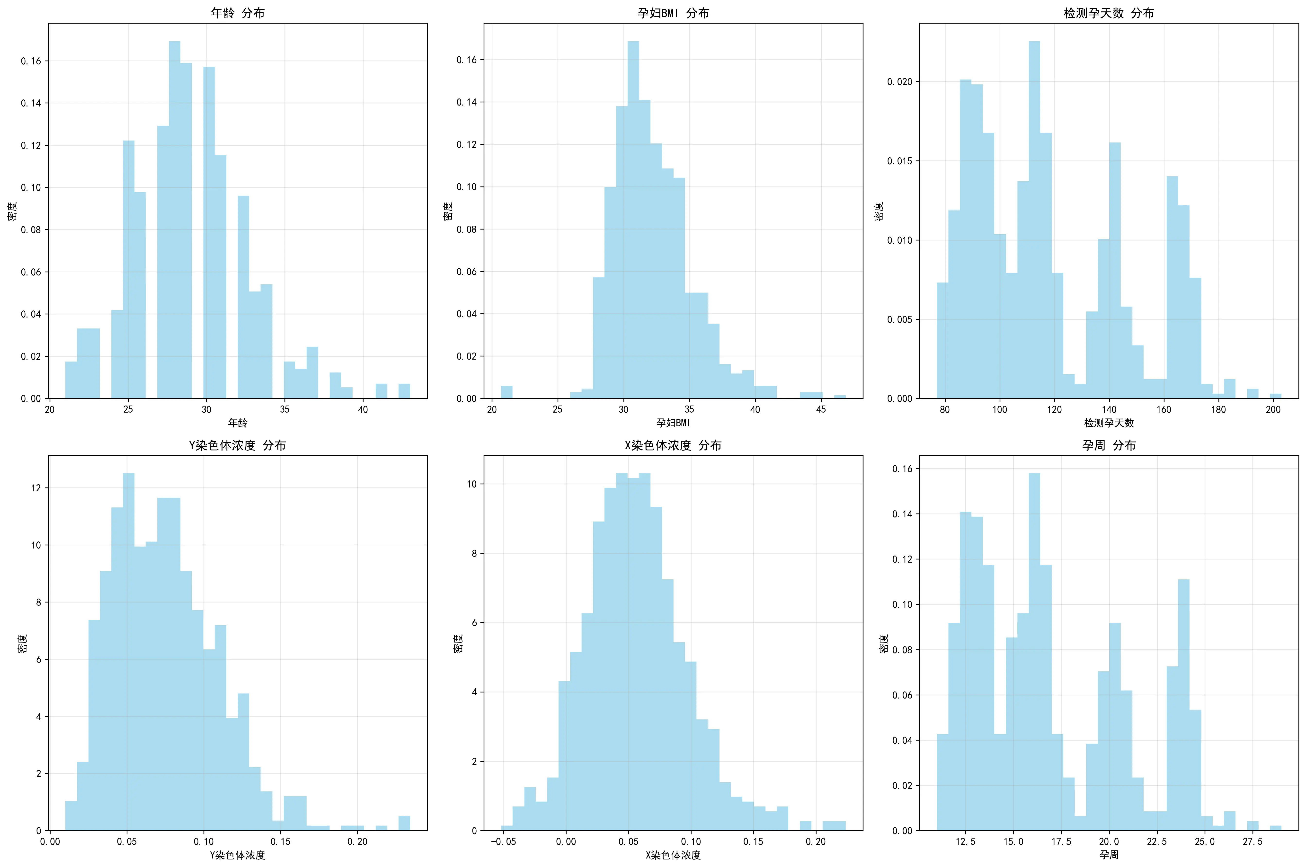
年龄、BMI、孕周以及Y染色体浓度等指标的分布揭示了样本的关键构成。通过分布柱状图可知,在年龄分布上,25-30岁年龄段的孕妇构成了最大的群体(超过400人),其次是30-35岁年龄段,整体呈现以青壮年育龄女性为主的典型分布。然而,在BMI方面,数据显示出本研究孕妇的一个显著特点:绝大多数孕妇(近770人)的BMI在27-37之间,少部分低于27或高于37。这表明本研究的样本群体主要由高BMI孕妇构成,为深入探究BMI对检测指标的影响提供了充足的数据支持。检测孕周无论按周还是按天排列,都呈现出明显的多峰形态,峰值大致出现在90天(约13周)、110天(约16周)和150天(约21周)附近。这表明样本的采集并非在孕期内均匀分布,而是集中在几个关键的临床检查时间点。作为本研究的核心因变量,Y染色体浓度的分布呈现出典型的严重右偏态。绝大多数样本的浓度值集中在较低的区间(0.05-0.10),仅有少数样本具有非常高的浓度值。X染色体的浓度分布呈现较标准的正态分布,峰值在0.05左右,但此数据对本题研究男胎的帮助不大。
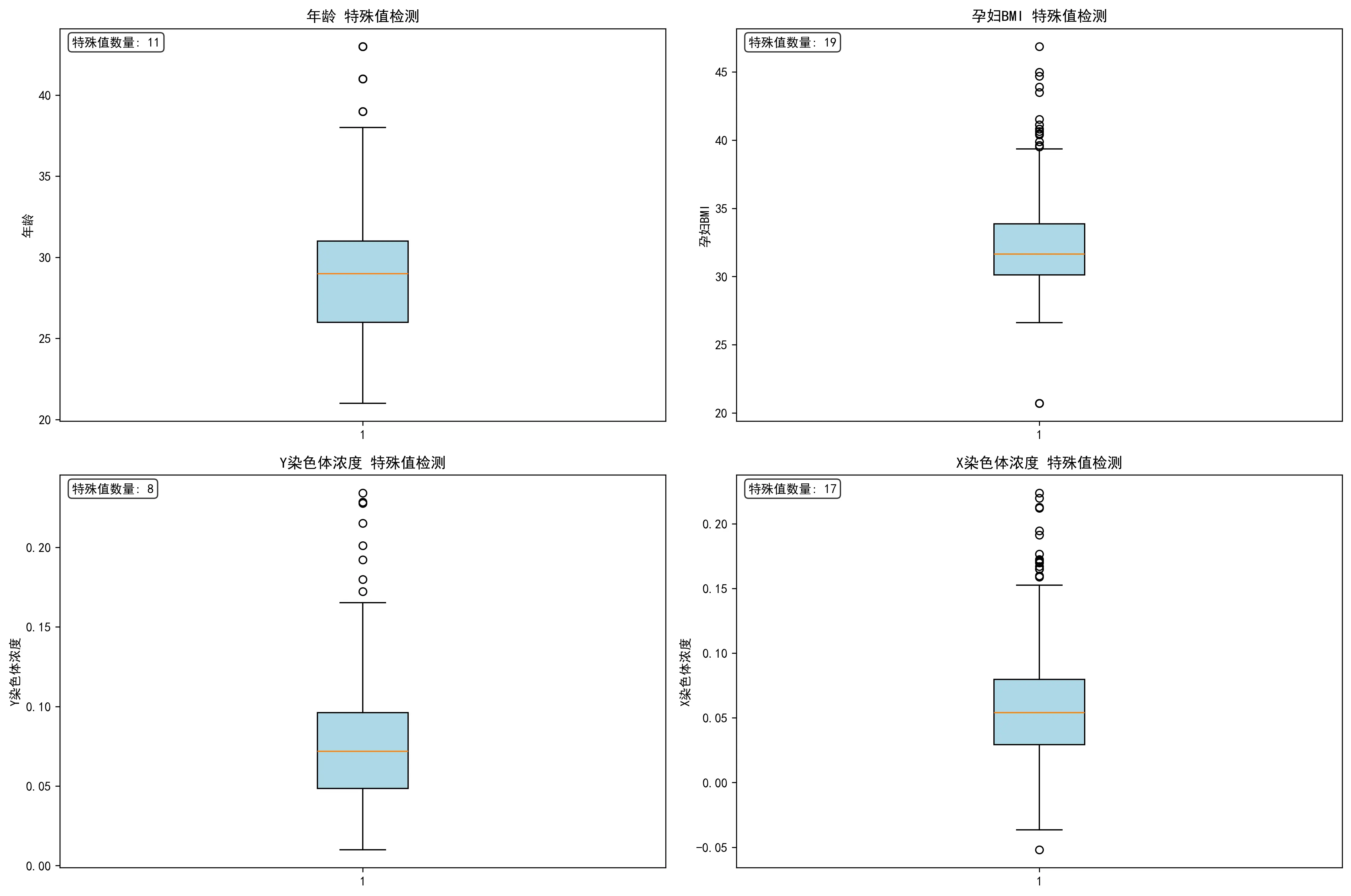
此外,本文对不同指标的特殊值进行了整理与探究。通过四张箱线图,直观地揭示了研究孕妇队列中关键变量的分布特征。它表明,该研究的样本主要由年龄集中在26-32岁的青壮年女性构成,但一个显著的特点是孕妇的身体质量指数(BMI)普遍偏高,且存在大量高值异常点。更重要的是,作为核心指标的Y染色体浓度呈现出典型的严重右偏态分布,即绝大多数样本的浓度值都集中在较低的区间,仅有少数样本具有非常高的浓度。
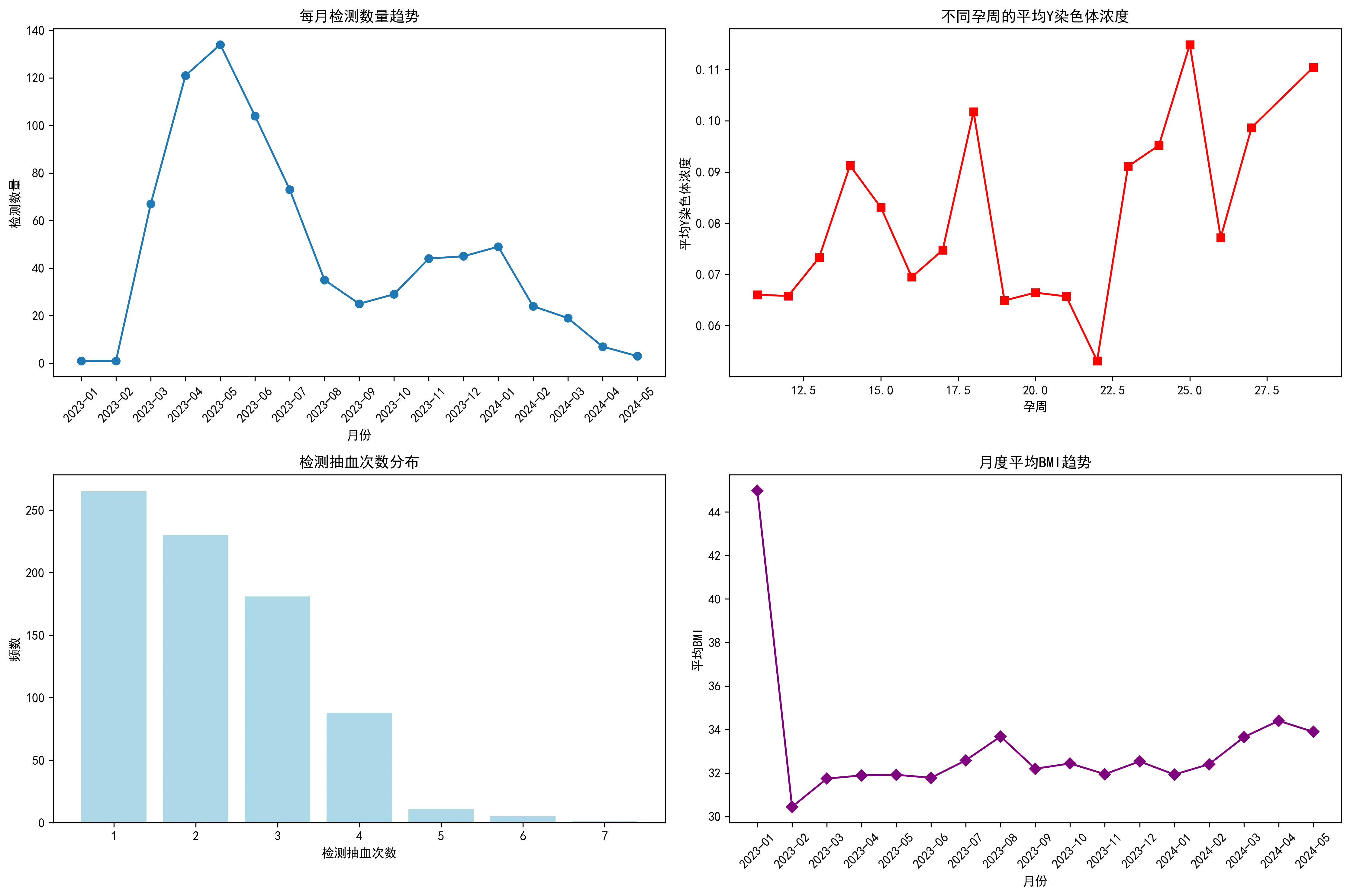
最后,从数据采集的时间趋势来看,从2023年1月至2024年5月,每月的检测数量呈现出一定的周期性波动,峰值出现在2023年春夏季。同时,孕妇的平均BMI在不同月份间也存在小幅波动,但未显示出与检测量同步的明确趋势。这些时间维度的信息有助于理解数据采集的背景,并评估潜在的时间混杂效应。此外,对孕妇的检测抽血次数分析显示,绝大多数孕妇仅进行1-2次检测,也为模型的构建提供了数据结构信息。
数据预处理
本题所提供的数据存在格式不统一、读取不方便、数据不合理等问题,在建模之前,需要先进行数据预处理,以确保分析结果更加科学、合理,模型建构更加稳定。本文对原始数据集进行了系统化的调整,包括对日期格式的统一、孕周格式的转换以及对无效数据的剔除。该流程旨在提升数据的一致性、完整性与可用性,从而减少噪声与偏差对模型性能的干扰。
日期格式的统一
原始数据中,不同的日期存在格式不统一的情况——"末次月经"的数据的年月日被“/”分开,而“检测日期”的数据的年月日被直接拼接在一起。为了读取数据更方便,本文将日期字段的数据都改成了“某年某月某日”的格式。具体示例如下:
日期格式统一示例
原始数据
改后数据
2023/5/20或20230520
2023年5月20日
孕周格式的转换
附件表格中的“检测孕周”字段的数据存在“周+天”的混合表示。本文将其全部换算成天数,方便数据的读取与比较。举例如下:
孕周格式转换示例
所以,初步的统计分析显示:样本覆盖的孕周主要集中在12周至20周之间,中位孕周约为14周;孕妇年龄分布广泛,平均年龄约31岁;BMI的中位数为23.5 k g / m 2 23.5kg/m^2 23.5 k g / m 2 > 30 k g / m 2 >30kg/m^2 > 30 k g / m 2
唯一比对读段数的筛选
在无创产前检测中,“唯一比对的读段数”是衡量数据有效性的重要指标,其能够唯一映射到参考基因组某一位置,反映了测序读段在参考基因组上的有效比对数量,还可有效减少因重复序列或错误比对导致的假阳性结构变异信号。本文对该指标进行了两个层面的筛选——读段数范围的界定以及读段数异常值的剔除。
(1)唯一比对读段数范围的界定
本文采用文献检索法 ,根据多篇方法学和临床研究,唯一比对读段数不应低于一个最低阈值,否则可能会因被检测基因片段过少而导致检测不准确。因此,依据文献内容,本文规定在检测第21号、18号、13号染色体浓度时,将0.15 × 覆盖度 ≈ 3 0.15\times\text{覆盖度}\approx3 0.15 × 覆盖度 ≈ 3
(2)唯一比对读段数异常值的剔除
附件中数据存在“唯一比对读段数”大于“原始读段数”的情况。因为前者是后者的一个子集,所以这在正常情况下是不可能发生的。因此,本文剔除了所有存在此情况的孕妇数据,一共71条。部分异常值数据如下:
唯一比对读段数异常值部分示例
序号
孕妇代码
原始读段数
唯一比对的读段数
690
A169
2132408
4395037
695
A171
2879248
3626619
696
A171
3636973
3737311
698
A171
3439440
3745489
经过上述步骤,数据集在时间格式、孕周表示及测序质量方面均实现了统一与优化。此外,本文对BMI值与身高、体重是否匹配进行了检验,发现全部匹配,无需调整。显著降低了因数据格式不一致或低质量样本引入的偏差风险,为后续的相关性分析、分组策略制定及数学模型构建奠定了坚实基础。
问题一的模型的建立和求解
数据整理与目标分析
本节旨在探究男胎样本中,哪些因素对母亲血浆中的胎儿Y染色体浓度产生影响。本文选取了孕周、孕妇BMI和孕妇年龄三个关键变量,希望评估它们与Y染色体浓度之间的独立关系。
针对预处理后的男胎检测数据,实行进一步的整理。对孕周数,仅提取周数作为数值,舍弃额外不满一周的天数;对需研究的四个变量,定义Y染色体浓度为Y Y Y X 1 X_1 X 1 X 2 X_2 X 2 X 3 X_3 X 3
为探究孕周、孕妇BMI及年龄对Y染色体浓度的独立影响,本研究构建了系统的统计分析模型。首先,通过正态性检验(Shapiro–Wilk检验)评估数据分布特性,结果显示所有关键变量均不服从正态分布。基于此,本文采用非参数的Spearman偏相关分析来衡量各变量间的单调关系强度。同时,为量化各因素的综合影响并建立预测模型,本文运用普通最小二乘法构建了多元线性回归模型,最终得到一个能够解释Y染色体浓度变化的数学方程。
正态性检验
Pearson相关系数的有效性依赖于变量服从正态分布的假设。为检验此假设,本文对四个核心变量采用Shapiro–Wilk检验进行正态性分析。
原假设H 0 H_0 H 0
备择假设H 1 H_1 H 1
Shapiro–Wilk检验结构
变量
检验p值
是否服从正态分布
Y染色体浓度
<0.0001
否(p<0.05)
检测孕周
<0.0001
否(p<0.05)
孕妇BMI
<0.0001
否(p<0.05)
年龄
<0.0001
否(p<0.05)
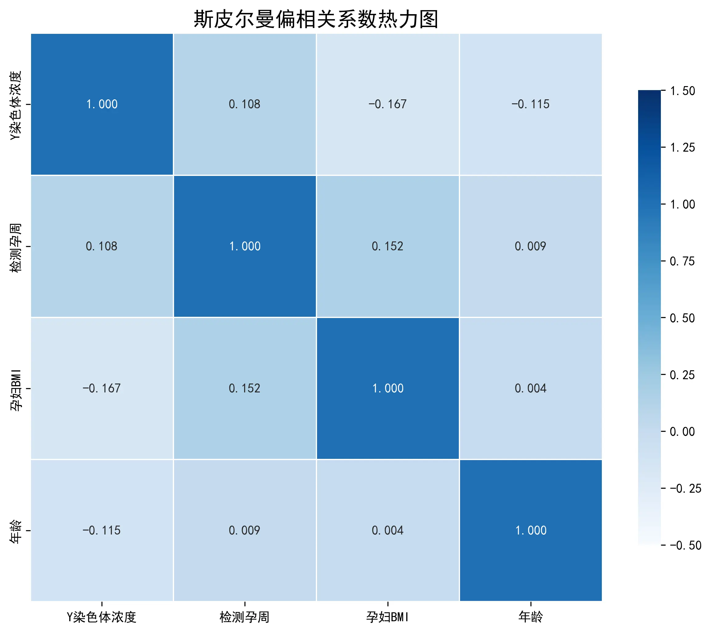
由此可知,所有变量的p值均远小于0.05的显著性水平。因此,本文拒绝了所有变量服从正态分布的假设。由于数据不满足正态性假设,使用Pearson偏相关分析可能会导致结果的偏差。因此,本文选择Spearman偏相关分析作为替代方法。Spearman相关是基于等级的非参数检验,它不要求数据服从特定的分布,对于非线性的关系也更为稳健,是处理当前数据的更优选择。
Spearman偏相关分析
Spearman偏相关分析结合了Spearman秩相关与偏相关的思想,既能处理非正态、非线性数据,又能在分析两个变量关系时控制其他变量的干扰。它不要求数据服从正态分布,适用于像本题数据一样分布未知的数据。(1)数据排序 :将所有涉及的变量( Y , X 1 , X 2 , X 3 ) (Y,X_1,X_2,X_3) ( Y , X 1 , X 2 , X 3 ) (2)计算偏相关系数 :当需要评估多个变量之间的独立性关系时,最系统的方法是使用逆矩阵法 一次性计算所有偏相关系数。
构建相关系数矩阵:首先,本文为所有涉及的变量( Y , X 1 , X 2 , X 3 ) (Y,X_1,X_2,X_3) ( Y , X 1 , X 2 , X 3 ) C \mathbf{C} C
C = ( 1 r Y X 1 r Y X 2 r Y X 3 r T 1 r X 1 X 2 r X 1 X 3 r X 2 Y r X 2 X 1 1 r X 2 X 3 r X 3 Y r X 3 X 1 r X 3 X 2 1 ) C = \begin{pmatrix}
1 & r_{YX_1} & r_{YX_2} & r_{YX_3} \\
r_{T} & 1 & r_{X_1X_2} & r_{X_1X_3} \\
r_{X_2Y} & r_{X_2X_1} & 1 & r_{X_2X_3} \\
r_{X_3Y} & r_{X_3X_1} & r_{X_3X_2} & 1
\end{pmatrix}
C = 1 r T r X 2 Y r X 3 Y r Y X 1 1 r X 2 X 1 r X 3 X 1 r Y X 2 r X 1 X 2 1 r X 3 X 2 r Y X 3 r X 1 X 3 r X 2 X 3 1
计算逆矩阵:计算该相关系数矩阵C \mathbf{C} C P = C − 1 P = C^{-1} P = C − 1
计算偏相关系数:任意两个变量 i i i j j j P \mathbf{P} P
r i j ⋅ Z = − p i j p i i p j j r_{ij \cdot Z} = - \frac{p_{ij}}{\sqrt{p_{ii} p_{jj}}}
r ij ⋅ Z = − p ii p jj p ij
例如,要计算Y染色体浓度(Y Y Y X 1 X_1 X 1 X 2 X_2 X 2 X 3 X_3 X 3 r Y X 1 ⋅ X 2 X 3 r_{YX_1 \cdot X_2X_3} r Y X 1 ⋅ X 2 X 3
r Y X 1 ⋅ X 2 X 3 = − p Y X 1 p Y Y p X 1 X 1 r_{YX_1 \cdot X_2X_3} = - \frac{p_{YX_1}}{\sqrt{p_{YY} p_{X_1X_1}}}
r Y X 1 ⋅ X 2 X 3 = − p YY p X 1 X 1 p Y X 1
这种方法为计算多变量控制下的偏相关系数提供了一个系统性的框架。其通过对相关矩阵求逆,一次性获得在控制其他变量影响后的全部成对相关系数,计算效率高、结果结构化且对称一致,适合多变量和高维数据分析;结合Spearman秩相关矩阵时,还能兼具抗异常值和非正态分布的稳健性。
(3)假设检验 :对计算出的每个偏相关系数进行显著性检验。
原假设H 0 H_0 H 0 ρ = 0 \rho = 0 ρ = 0
备择假设H 1 H_1 H 1 ρ ≠ 0 \rho \neq 0 ρ = 0
t统计量:t = r n − k − 2 1 − r 2 t = r \sqrt{\frac{n - k - 2}{1 - r^2}} t = r 1 − r 2 n − k − 2
自由度:d f = n − k − 2 df = n - k - 2 df = n − k − 2 n n n k k k
Spearman偏相关系数矩阵 (基于秩次)
Y染色体浓度
检测孕周
孕妇BMI
年龄
Y染色体浓度 1.000000
0.086422
-0.140745
-0.095451
检测孕周 0.086422
1.000000
0.145435
-0.013050
孕妇BMI -0.140745
0.145435
1.000000
0.027144
年龄 -0.095451
-0.013050
0.027144
1.000000
结果显示:
(1)Y染色体浓度与检测孕周(r = 0.086 r=0.086 r = 0.086 正相关 关系。
(2)Y染色体浓度与孕妇BMI(r = − 0.141 r=-0.141 r = − 0.141 负相关 关系。这是三个因素中相关性最强的一个。
(3)Y染色体浓度与孕妇年龄(r = − 0.095 r=-0.095 r = − 0.095 负相关 关系。
通过对相关性系数的分析与对比,得出结论:孕周与Y染色体浓度呈正相关,在BMI和年龄相近的情况下,孕周越长,Y染色体浓度越高;孕妇BMI与Y染色体浓度呈负相关。在孕周和年龄相近的情况下,孕妇BMI越高,Y染色体浓度越低,这可能与“稀释效应”有关;孕妇年龄与Y染色体浓度呈负相关。在孕周和BMI相近的情况下,孕妇年龄越大,Y染色体浓度越低。
多元线性回归模型的建立与求解
根据上述分析,为量化孕周、孕妇BMI、孕妇年龄三个自变量与Y染色体浓度的关系模型,本文采用多元线性回归,其能够同时考虑多个自变量对因变量的影响,在控制其他因素的情况下量化各变量的独立贡献,从而更全面、准确地解释因变量的变化规律;其可通过回归系数、显著性检验和拟合优度等指标评估模型的统计可靠性与预测能力。本题中,该模型不仅能对变量间的相关性情况进行验证,还能量化其影响,更深层次地评估变量间的关联情况。
多元线性回归模型的建立
(1)模型设定
根据题意,结合模型可基本假设因变量Y Y Y X 1 , X 2 , X 3 X_1, X_2, X_3 X 1 , X 2 , X 3 ϵ \epsilon ϵ
Y i = β 0 + β 1 X i 1 + β 2 X i 2 + β 3 X i 3 + ϵ i Y_i = \beta_0 + \beta_1 X_{i1} + \beta_2 X_{i2} + \beta_3 X_{i3} + \epsilon_i
Y i = β 0 + β 1 X i 1 + β 2 X i 2 + β 3 X i 3 + ϵ i
其中:
i i i i i i Y i Y_i Y i i i i X i 1 , X i 2 , X i 3 X_{i1}, X_{i2}, X_{i3} X i 1 , X i 2 , X i 3 β 0 \beta_0 β 0 Y Y Y β 1 , β 2 , β 3 \beta_1, \beta_2, \beta_3 β 1 , β 2 , β 3 β j \beta_j β j X j X_j X j Y Y Y ϵ i \epsilon_i ϵ i Y i Y_i Y i
(2)模型拟合:最小二乘法
由于总体系数β j \beta_j β j 普通最小二乘法 来寻找最佳的系数估计值。该方法的目标是找到一组系数估计值β ^ 0 , β ^ 1 , β ^ 2 , β ^ 3 \hat{\beta}_0, \hat{\beta}_1, \hat{\beta}_2, \hat{\beta}_3 β ^ 0 , β ^ 1 , β ^ 2 , β ^ 3
Y ^ i = β ^ 0 + β ^ 1 X i 1 + β ^ 2 X i 2 + β ^ 3 X i 3 \hat{Y}_i = \hat{\beta}_0 + \hat{\beta}_1 X_{i1} + \hat{\beta}_2 X_{i2} + \hat{\beta}_3 X_{i3}
Y ^ i = β ^ 0 + β ^ 1 X i 1 + β ^ 2 X i 2 + β ^ 3 X i 3
其中 Y ^ i \hat{Y}_i Y ^ i e i e_i e i
e i = Y i − Y ^ i e_i = Y_i - \hat{Y}_i
e i = Y i − Y ^ i
最小二乘法的目标是最小化所有残差的平方和 (SSR):
SSR = ∑ i = 1 n e i 2 = ∑ i = 1 n ( Y i − Y ^ i ) 2 = ∑ i = 1 n ( Y i − β ^ 0 − β ^ 1 X i 1 − β ^ 2 X i 2 − β ^ 3 X i 3 ) 2 \text{SSR} = \sum_{i=1}^{n} e_i^2 = \sum_{i=1}^{n} (Y_i - \hat{Y}_i)^2 = \sum_{i=1}^{n} (Y_i - \hat{\beta}_0 - \hat{\beta}_1 X_{i1} - \hat{\beta}_2 X_{i2} - \hat{\beta}_3 X_{i3})^2
SSR = i = 1 ∑ n e i 2 = i = 1 ∑ n ( Y i − Y ^ i ) 2 = i = 1 ∑ n ( Y i − β ^ 0 − β ^ 1 X i 1 − β ^ 2 X i 2 − β ^ 3 X i 3 ) 2
其中 n n n β ^ j \hat{\beta}_j β ^ j β ^ 0 , β ^ 1 , β ^ 2 , β ^ 3 \hat{\beta}_0, \hat{\beta}_1, \hat{\beta}_2, \hat{\beta}_3 β ^ 0 , β ^ 1 , β ^ 2 , β ^ 3 Y \mathbf{Y} Y n × 1 n \times 1 n × 1 X \mathbf{X} X n × 4 n \times 4 n × 4 β \boldsymbol{\beta} β 4 × 1 4 \times 1 4 × 1 η ^ \hat{\boldsymbol{\eta}} η ^ β \boldsymbol{\beta} β
Y = ( Y 1 Y 2 ⋮ Y n ) , X = ( 1 X 11 X 12 X 13 1 X 21 X 22 X 23 ⋮ ⋮ ⋮ ⋮ 1 X n 1 X n 2 X n 3 ) , β ^ = ( β ^ 0 β ^ 1 β ^ 2 β ^ 3 ) \mathbf{Y} = \begin{pmatrix}
Y_1 \\ Y_2 \\ \vdots \\ Y_n \end{pmatrix}, \quad
\mathbf{X} = \begin{pmatrix}
1 & X_{11} & X_{12} & X_{13} \\
1 & X_{21} & X_{22} & X_{23}\\
\vdots & \vdots & \vdots & \vdots \\ 1 & X_{n1} & X_{n2} & X_{n3} \end{pmatrix},\quad \hat{\boldsymbol{\beta}} = \begin{pmatrix} \hat{\beta}_0 \\ \hat{\beta}_1 \\ \hat{\beta}_2 \\ \hat{\beta}_3 \end{pmatrix}
Y = Y 1 Y 2 ⋮ Y n , X = 1 1 ⋮ 1 X 11 X 21 ⋮ X n 1 X 12 X 22 ⋮ X n 2 X 13 X 23 ⋮ X n 3 , β ^ = β ^ 0 β ^ 1 β ^ 2 β ^ 3
SSR可以表示为:
SSR = ( Y − X β ^ ) T ( Y − X β ^ ) \text{SSR} = (\mathbf{Y} - \mathbf{X}\hat{\boldsymbol{\beta}})^T (\mathbf{Y} - \mathbf{X}\hat{\boldsymbol{\beta}})
SSR = ( Y − X β ^ ) T ( Y − X β ^ )
通过求解 ∂ ( SSR ) ∂ β ^ = 0 \frac{\partial(\text{SSR})}{\partial \hat{\boldsymbol{\beta}}} = 0 ∂ β ^ ∂ ( SSR ) = 0
( X T X ) β ^ = X T Y (\mathbf{X}^T \mathbf{X}) \hat{\boldsymbol{\beta}} = \mathbf{X}^T \mathbf{Y}
( X T X ) β ^ = X T Y
最终,本文可以解出系数的估计向量 β ^ \hat{\boldsymbol{\beta}} β ^
β ^ = ( X T X ) − 1 X T Y \hat{\boldsymbol{\beta}} = (\mathbf{X}^T \mathbf{X})^{-1} \mathbf{X}^T \mathbf{Y}
β ^ = ( X T X ) − 1 X T Y
本次模型构建旨在量化检测孕周、孕妇BMI及年龄对Y染色体浓度的独立影响。为此,本文采用了双重分析策略:
多元线性回归模型的求解
具体的系数估计值:
{ β ^ 0 = 0.1384 β ^ 1 (检测孕周) = 0.0002 β ^ 2 (孕妇BMI) = − 0.0016 β ^ 3 (年龄) = − 0.0010 \begin{cases}
\hat{\beta}_0 = 0.1384\\
\hat{\beta}_1\text{(检测孕周)} = 0.0002\\
\hat{\beta}_2 \text{(孕妇BMI)} = -0.0016\\
\hat{\beta}_3 \text{(年龄)} = -0.0010
\end{cases}
⎩ ⎨ ⎧ β ^ 0 = 0.1384 β ^ 1 (检测孕周) = 0.0002 β ^ 2 (孕妇 BMI ) = − 0.0016 β ^ 3 (年龄) = − 0.0010
将这些估计值代入样本回归方程,得到最终的拟合模型:
Y染色体浓度 ^ = 0.1384 + 0.0002 × ( 检测孕周 ) − 0.0016 × ( 孕妇BMI ) − 0.0010 × ( 年龄 ) \widehat{\text{Y染色体浓度}} = 0.1384 + 0.0002 \times (\text{检测孕周}) - 0.0016 \times (\text{孕妇BMI}) - 0.0010 \times (\text{年龄})
Y 染色体浓度 = 0.1384 + 0.0002 × ( 检测孕周 ) − 0.0016 × ( 孕妇 BMI ) − 0.0010 × ( 年龄 )
该方程就是对Y染色体浓度进行预测的数学模型。例如,对于一个检测孕周为20周、BMI为25、年龄为30岁的孕妇,其Y染色体浓度的预测值为:
Y ^ = 0.1384 + 0.0002 × 20 − 0.0016 × 25 − 0.0010 × 30 = 0.0724 \hat{Y} = 0.1384 + 0.0002 \times 20 - 0.0016 \times 25 - 0.0010 \times 30 = 0.0724
Y ^ = 0.1384 + 0.0002 × 20 − 0.0016 × 25 − 0.0010 × 30 = 0.0724
这个过程清晰地展示了如何从理论模型出发,利用OLS方法和样本数据,最终得到一个可用于解释和预测的、具体的数学方程。
模型评估
本文中的多元线性回归模型的R 2 = 0.045 R^2=0.045 R 2 = 0.045 1.66 × 10 − 8 1.66\times10^{-8} 1.66 × 1 0 − 8
本次构建的回归模型在统计学上是高度显著的。模型的F统计量对应的p值(1.66 × 10 − 8 1.66\times10^{-8} 1.66 × 1 0 − 8
从模型系数来看,所有纳入的自变量——检测孕周、孕妇BMI和年龄——均为统计上非常显著的预测因子。具体而言,检测孕周与Y染色体浓度呈显著正相关,而孕妇BMI和年龄则与其呈显著负相关。这意味着,在控制了其他变量后,孕周越长、BMI越低、年龄越轻的孕妇,其血浆中胎儿Y染色体浓度倾向于更高。
然而,模型的实际解释能力非常有限。R 2 R^2 R 2 R 2 R^2 R 2 R 2 R^2 R 2
综上所述,该模型成功地识别出了几个影响Y染色体浓度的关键统计学指标及其影响方向,为理解这一生理现象提供了有价值的线索。但其较低的R平方值也明确警示本文,Y染色体浓度是一个受多重复杂因素共同调控的指标,孕妇检测孕周、孕妇BMI、孕妇年龄这三个指标对Y染色体浓度的影响的贡献很小,但显著性很强。
问题二的模型的建立和求解
为解决传统BMI分组在预测检测成功率方面区分度不足的问题,本研究构建了一套数据驱动的监督式分箱。该方法首先将问题转化为一个生存分析框架,通过区间删失方法处理纵向检测数据中“指标达标”事件发生时间的不确定性。随后,本文采用多重插补技术来应对区间删失带来的问题,并在每个插补数据集上拟合带B样条变换的Cox比例风险模型,为每个BMI值预测一个“指标达标孕周”。最后,以该预测孕周为监督信号,通过CART回归树算法以数据驱动的方式寻找最优的BMI分组切点,并结合剪枝与最小样本量等策略保证分箱的稳健性。最后,在每个分组内,使用Kaplan–Meier方法估计生存曲线和推荐时间点(t95),再经跨组保序和半周圆整后得出最终推荐时点。为了分析检测误差对结果的影响,本文通过“模糊区间”分析与“加噪蒙特卡洛”分析两种独立的敏感性分析来评估模型的稳健性,最终确认了模型在面对测量误差时的稳健性与可靠性。
数据探索性分析(EDA)
在正式构建监督式分箱模型之前,本文首先对原始数据进行了探索性分析(EDA),以评估传统BMI分组的预测能力。通过绘制BMI与关键检测指标的散点图并叠加LOWESS平滑曲线,探究BMI与关键检测指标的相关性情况,这为后续建模提供了理论依据。随后,本文将孕妇按照常规的的BMI标准(例如[20,28),[28,32),[32,36),[36,40),40 以上)进行分组,并对各组分别进行了KM生存分析,以比较其“指标达标”事件的发生率曲线。分析结果显示,尽管不同分组的KM曲线呈现出一定的分离趋势,但各曲线间区分度不足,甚至存在交叉现象。这一发现明确地揭示了传统分组方法无法有效且稳定地对风险进行分层,从而凸显了采用数据驱动的监督式学习方法来寻找最优风险分割点的必要性。
探索性数据分析结果
对本题所给的原始分组样例进行分析后,得出了孕妇BMI值与关键检测指标之间的关系,如下图所示。图中包含了所有数据点的散点图,以及一条LOWESS平滑拟合曲线。曲线清晰地揭示了BMI与关键检测指标之间存在负相关趋势。即随着BMI的增高,可能导致检测成功的关键生物指标浓度趋于下降,这是后续建模的理论基础。其次,基于传统的BMI分组,绘制了KM生存曲线。这里的“生存”事件可以理解为“未发生检测误差”。
图中各曲线存在一定的分离趋势,表明不同BMI分组的检测误差率确实存在差异。然而,曲线之间的分离度存在交叉,说明简单的BMI分组不足以清晰、稳定地划分风险等级,这凸显了后续采用“监督式分箱”的必要性。
阈值的设定
在本研究中,阈值 c 是定义核心分析事件的基石。它代表了一个关键的临床或技术判断标准,用于判定某次检测的测量值 y i j y_{ij} y ij y i j > = c y_{ij} >= c y ij >= c T i T_i T i L i , R i L_i, R_i L i , R i c l , c u c_l, c_u c l , c u
令原始行级观测集合为R = { ( i , j ) : ( p i d i , t i j , y i j , B M I i ) } \mathcal{R}=\{(i,j): (\mathrm{pid}_i, t_{ij}, y_{ij}, \mathrm{BMI}_i )\} R = {( i , j ) : ( pid i , t ij , y ij , BMI i )} p i d i \mathrm{pid}_i pid i i i i i = 1 , … , n i=1,\dots,n i = 1 , … , n c c c h i t i j = 1 { y i j ≥ c } \mathrm{hit}_{ij} = \mathbf{1}\{y_{ij} \ge c\} hit ij = 1 { y ij ≥ c } T i T_i T i [ c ℓ , c u ] [c_\ell,c_u] [ c ℓ , c u ]
(1)若存在最早的 j j j y i j > c u y_{ij} > c_u y ij > c u R i = w i j R_i=w_{ij} R i = w ij L i L_i L i R i R_i R i
(2)若全序列中没有 y i j > c u y_{ij} > c_u y ij > c u L i = max j w i j L_i=\max_j w_{ij} L i = max j w ij
多重插补方法(MI)
由于本文无法观测到每位孕妇检测指标首次“达标”的确切孕周,只能确定它发生于某两次检测之间的时间窗口 [L i , R i L_i, R_i L i , R i M M M T i T_i T i M M M M M M
为处理“不确定”的达标时间,根据区间化规则,对第 i i i h i t i k = 1 \mathrm{hit}_{ik}=1 hit ik = 1 k k k j ∗ < k j^*<k j ∗ < k h i t i j ∗ = 0 \mathrm{hit}_{ij^*}=0 hit i j ∗ = 0 L i = w i , j ∗ , R i = w i , k , ctype i = 区间删失 L_i=w_{i,j^*},\quad R_i=w_{i,k},\quad
\text{ctype}_i=\text{区间删失} L i = w i , j ∗ , R i = w i , k , ctype i = 区间删失 L i = w l b (常设为检测下限,例如 6 周) , R i = w i , k , ctype i = 左删失 L_i = w_{\mathrm{lb}}\ \text{(常设为检测下限,例如 6 周)},\quad R_i = w_{i,k},\quad \text{ctype}_i=\text{左删失} L i = w lb ( 常设为检测下限,例如 6 周 ) , R i = w i , k , ctype i = 左删失 L i = w i , max , R i = + ∞ , ctype i = 右删失 L_i = w_{i,\max},\quad R_i = +\infty,\quad \text{ctype}_i=\text{右删失} L i = w i , m a x , R i = + ∞ , ctype i = 右删失
然后,对每个左删失样本做M M M 插补 ,构造完整时间样本:
(1)均匀插补: T i ( m ) ∼ U n i f ( L i , R i ) , m = 1 , … , M T_i^{(m)} \sim \mathrm{Unif}(L_i,R_i),\quad m=1,\dots,M T i ( m ) ∼ Unif ( L i , R i ) , m = 1 , … , M
(2)**截断指数插补:**给定尺度参数 θ > 0 \theta>0 θ > 0
f ( t ) = ( 1 / θ ) e − ( t − L i ) / θ 1 − e − ( R i − L i ) / θ , t ∈ ( L i , R i ) , f(t) = \frac{(1/\theta) e^{-(t-L_i)/\theta}}{1 - e^{-(R_i-L_i)/\theta}},\quad t\in(L_i,R_i),
f ( t ) = 1 − e − ( R i − L i ) / θ ( 1/ θ ) e − ( t − L i ) / θ , t ∈ ( L i , R i ) ,
其逆变换采样为
t = − θ ln ( 1 − U ( 1 − e − ( R i − L i ) / θ ) ) + L i , U ∼ U n i f ( 0 , 1 ) , t = -\theta \ln\big(1 - U (1-e^{-(R_i-L_i)/\theta})\big) + L_i,\quad U\sim\mathrm{Unif}(0,1),
t = − θ ln ( 1 − U ( 1 − e − ( R i − L i ) / θ ) ) + L i , U ∼ Unif ( 0 , 1 ) ,
(3)**自适应插补:**先按 BMI 分组计算每组左删失比例 r g r_g r g r g r_g r g τ \tau τ L i ← 10 L_i\leftarrow 10 L i ← 10 T i = L i T_i=L_i T i = L i δ i = 0 \delta_i=0 δ i = 0 M M M D ( m ) \mathcal{D}^{(m)} D ( m )
Cox模型的建立与分位时间预测
在本研究中,Cox比例风险模型是连接孕妇BMI与其检测指标“达标”事件风险的核心预测引擎。由于BMI与“达标”风险之间的关系可能并非简单的线性,本文不直接使用原始BMI值,而是采用B样条对其进行变换。B样条能将BMI灵活地表示为一组分段多项式基函数,从而有效捕捉两者间复杂的非线性模式。在经过多重插补后,本文在每个插补数据集上独立拟合一个Cox模型,该模型以BMI的B样条变换结果作为协变量,用以估计每个BMI值对应的“达标”瞬时风险。通过该模型,能为每位孕妇计算出其个体化的生存函数S i ^ ( t ) \hat{S_i}(t) S i ^ ( t ) T i ^ \hat{T_i} T i ^ D ( m ) \mathcal{D}^{(m)} D ( m ) X i X_i X i λ i ( t ) = λ 0 ( t ) exp ( β ⊤ X i ) \lambda_i(t) = \lambda_0(t) \exp(\beta^\top X_i) λ i ( t ) = λ 0 ( t ) exp ( β ⊤ X i ) T \mathcal{T} T S ^ i ( m ) ( t ) = S ^ 0 ( m ) ( t ) exp ( β ⊤ X i ) \widehat S_i^{(m)}(t) = \widehat S_0^{(m)}(t)^{\exp(\beta^\top X_i)} S i ( m ) ( t ) = S 0 ( m ) ( t ) e x p ( β ⊤ X i ) p p p p = 0.95 p=0.95 p = 0.95 p p p
T ^ i , p ( m ) = inf { t ∈ T : S ^ i ( m ) ( t ) ≤ 1 − p } ; \widehat T_{i,p}^{(m)} = \inf\{t\in\mathcal{T}:\ \widehat S_i^{(m)}(t) \le 1-p\};
T i , p ( m ) = inf { t ∈ T : S i ( m ) ( t ) ≤ 1 − p } ;
跨插补聚合(本文取中位数)得到最终预测:T ^ i , p = m e d i a n m = 1 M T ^ i , p ( m ) \widehat T_{i,p} = \mathrm{median}_{m=1}^M \widehat T_{i,p}^{(m)} T i , p = median m = 1 M T i , p ( m )
曲线单调化
为保证 BMI 增加时预测不减少,令样本按 BMI 升序排列为 x ( 1 ) ≤ ⋯ ≤ x ( n ) x_{(1)}\le\dots\le x_{(n)} x ( 1 ) ≤ ⋯ ≤ x ( n ) y ( i ) = T ^ ( i ) , p y_{(i)}=\widehat T_{(i),p} y ( i ) = T ( i ) , p y ~ ( i ) \widetilde y_{(i)} y ( i )
y ~ = arg min y ~ ( 1 ) ≤ ⋯ ≤ y ~ ( n ) ∑ i = 1 n ( y ( i ) − y ~ ( i ) ) 2 \widetilde y = \arg\min_{\widetilde y_{(1)}\le\cdots\le\widetilde y_{(n)}} \sum_{i=1}^n (y_{(i)} - \widetilde y_{(i)})^2
y = arg y ( 1 ) ≤ ⋯ ≤ y ( n ) min i = 1 ∑ n ( y ( i ) − y ( i ) ) 2
由单调回归求解,求得y i m o n o y_i^{\mathrm{mono}} y i mono
回归树模型与KM估计
单变量回归树是一种决策树回归模型,用于预测一个连续型目标变量,其输入只有一个特征变量。它通过递归地划分输入变量的取值区间,在每个区间内用一个常数值来进行预测。以单变量 BMI 为自变量拟合回归树,来拟合 y m o n o y^{\mathrm{mono}} y mono K K K { I g } g = 1 K \{\mathcal{I}_g\}_{g=1}^K { I g } g = 1 K y m o n o y^{\mathrm{mono}} y mono ≥ w min \ge w_{\min} ≥ w m i n ≥ n min \ge n_{\min} ≥ n m i n K = 4 K=4 K = 4
M A E = 1 n ∑ i = 1 n ∣ y i − y ^ g ( i ) ∣ \mathrm{MAE} = \frac{1}{n} \sum_{i=1}^n | y_i - \widehat y_{g(i)} |
MAE = n 1 i = 1 ∑ n ∣ y i − y g ( i ) ∣
其中 y ^ g \widehat y_{g} y g
在最终分组下对每组做KM估计,并估计第p p p t g , p t_{g,p} t g , p g g g S ^ g ( t ) \widehat S_g(t) S g ( t ) p p p
t g , p = inf { t : S ^ g ( t ) ≤ 1 − p } t_{g,p} = \inf\{t: \widehat S_g(t) \le 1-p\}
t g , p = inf { t : S g ( t ) ≤ 1 − p }
在 MI 环境下,对每个插补集分别计算 t g , p ( m ) t_{g,p}^{(m)} t g , p ( m ) 回归树分组与KM估计结果
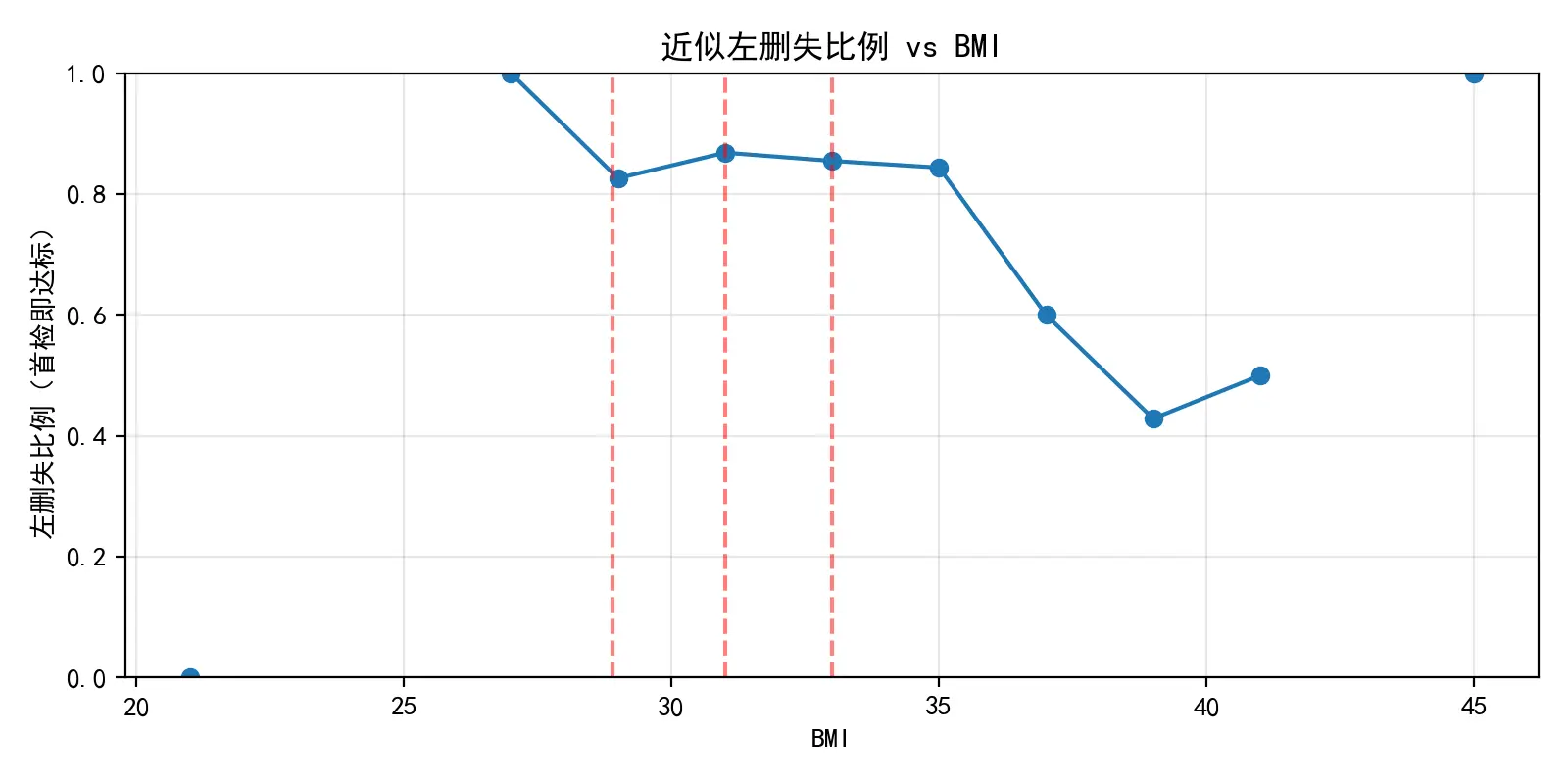
利用单变量回归树模型,得到最佳BMI切点数值及各组孕妇的最佳检测时点。
最佳BMI分组及检测时点
BMI组别
人数
最佳检测周数
29.0及以下
32
18.0
{}[29.0,31.1)
89
18.5
{}[31.1,33.2)
68
19.5
33.2及以上
68
23.0
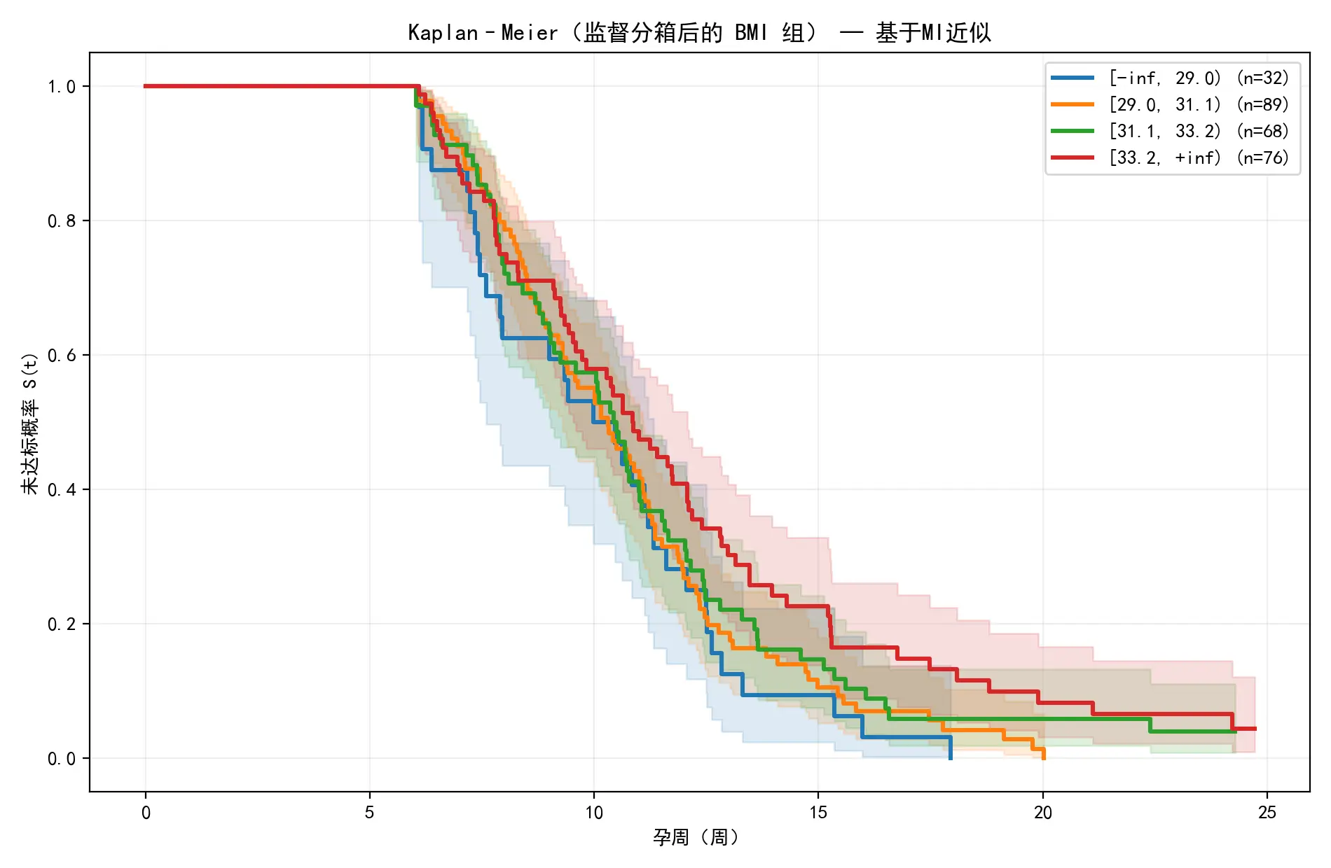
对此分组结果重新绘制KM生存曲线,如下图所示:
与原始分组的KM曲线相比,此图中的各组曲线分离得更为清晰、层次分明,高风险组的“无误差率”显著低于低风险组。这证明本文的算法成功地找到了能最大化风险差异的BMI阈值。
模型评估
log-rank对数秩检验
在确定分组后,为量化各组别之间的区分度,本文还对相邻两个风险组的KM生存曲线进行了对数秩检验,得到其p值。如下表所示:
对数秩检验p值
组别比较
p m p_m p m p f p_f p f
29及以下与[29.0,31.1)
0.349
0.638
\relax[29.0,31.1)与[31.1,33.2)
0.168
0.302
\relax[31.1,33.2)与33.2及以上
0.093
0.051
由此可知,p值并非极小,这表明相邻风险组之间在KM生存曲线上的差异并非极其显著,有偶然因素掺杂。
敏感性分析
为探究检测误差对分组结果和最佳 NIPT时点的影响,本文分别进行了两个分析实验,分别测量噪声和模糊阈值对结果的影响。
首先是测量噪声的蒙特卡洛模拟。在每次模拟 b = 1 , … , B b=1,\dots,B b = 1 , … , B
y ~ i j ( b ) = y i j + ε i j ( b ) , ε i j ( b ) ∼ N ( 0 , σ 2 ) , σ = 0.01. \tilde y_{ij}^{(b)} = y_{ij} + \varepsilon_{ij}^{(b)},\qquad \varepsilon_{ij}^{(b)}\sim\mathcal{N}(0,\sigma^2),\sigma=0.01.
y ~ ij ( b ) = y ij + ε ij ( b ) , ε ij ( b ) ∼ N ( 0 , σ 2 ) , σ = 0.01.
对每次扰动数据,重复区间化、MI(M M M K = 4 K=4 K = 4
( C ( b ) , t 1 , p ( b ) , … , t K , p ( b ) ) . (\mathcal{C}^{(b)},\; t_{1,p}^{(b)},\dots,t_{K,p}^{(b)} ).
( C ( b ) , t 1 , p ( b ) , … , t K , p ( b ) ) .
收集成功次样本的经验分布以估计切点与组内推荐的不确定性(均值、方差、置信区间、直方图等)。
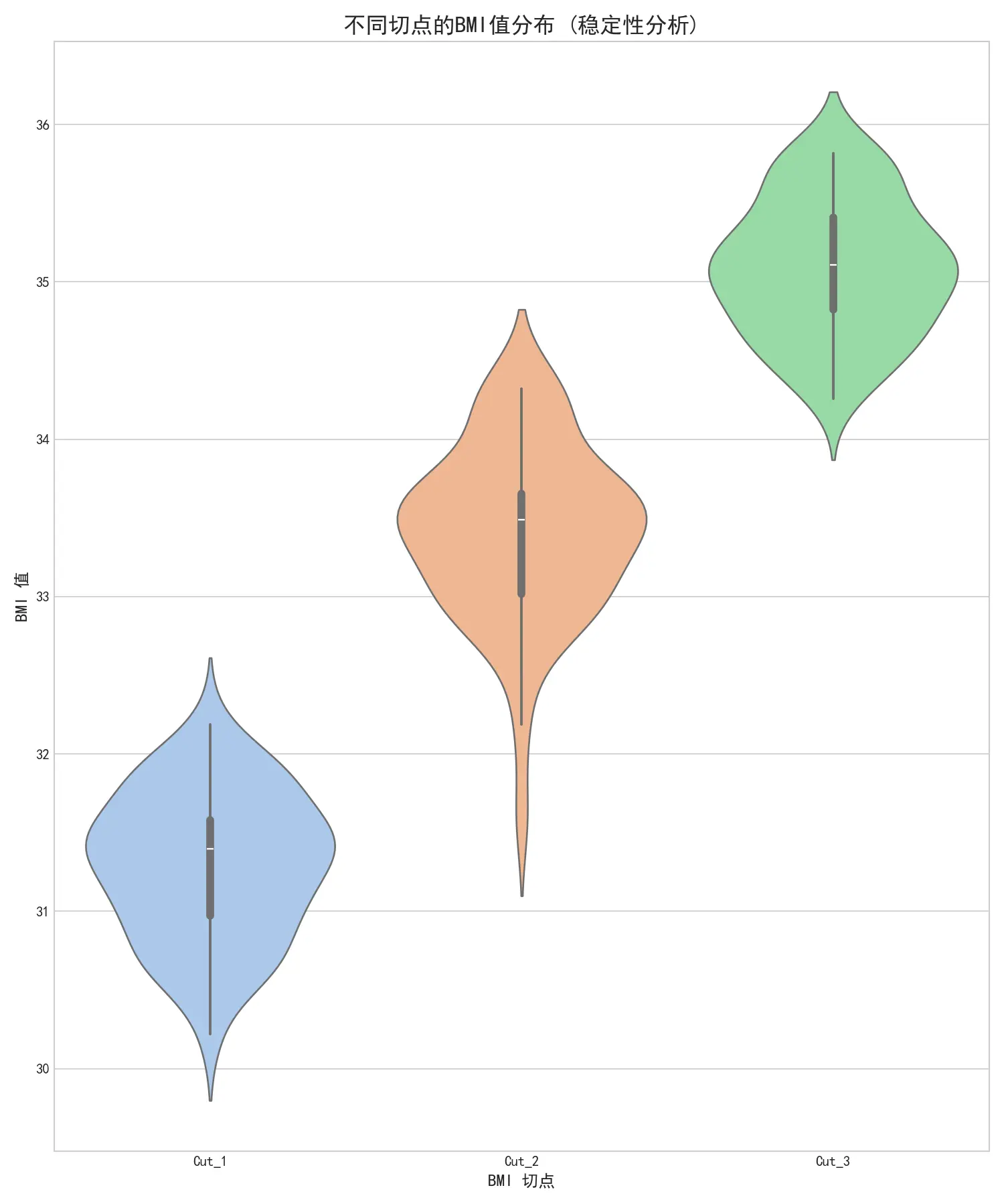
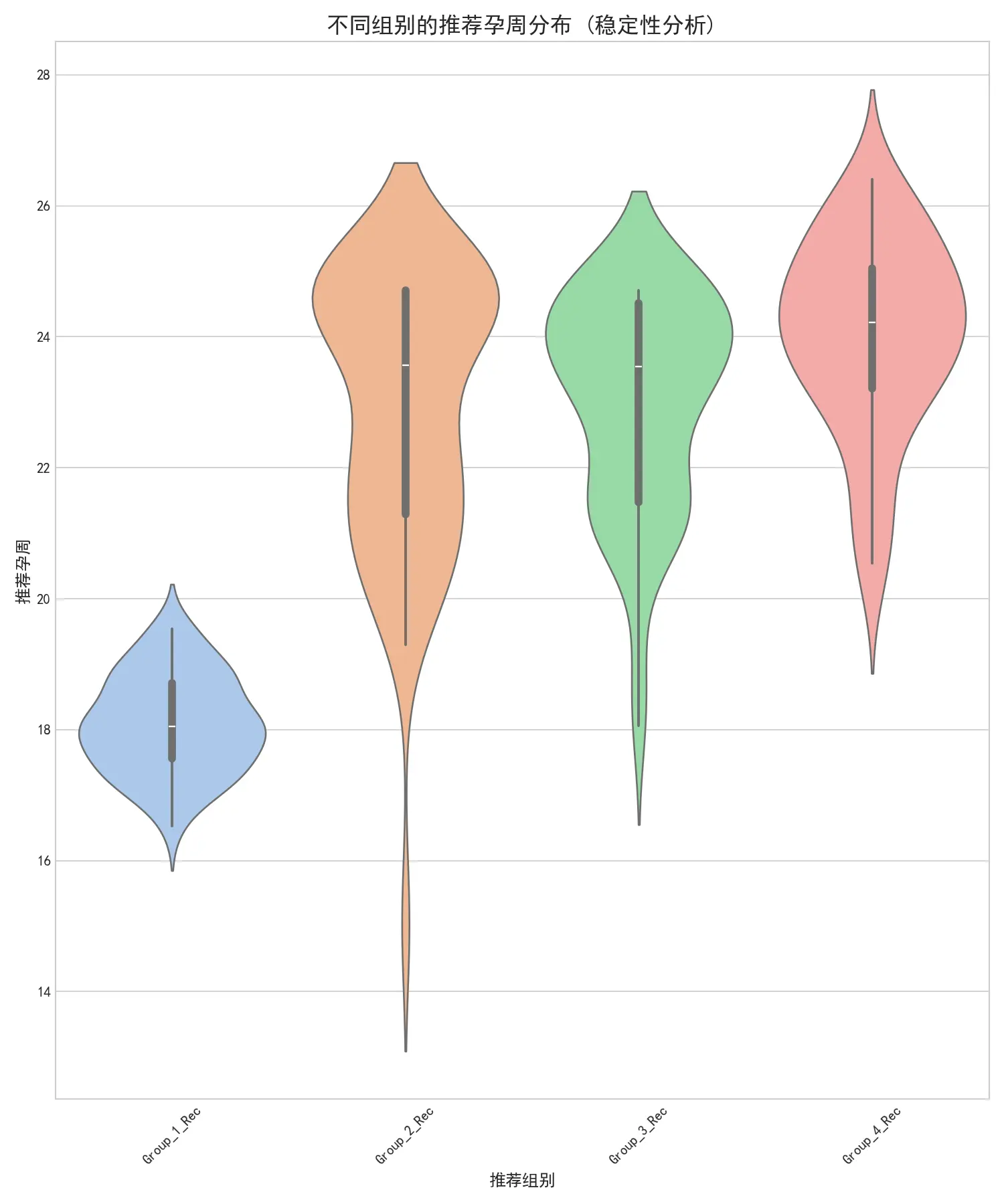
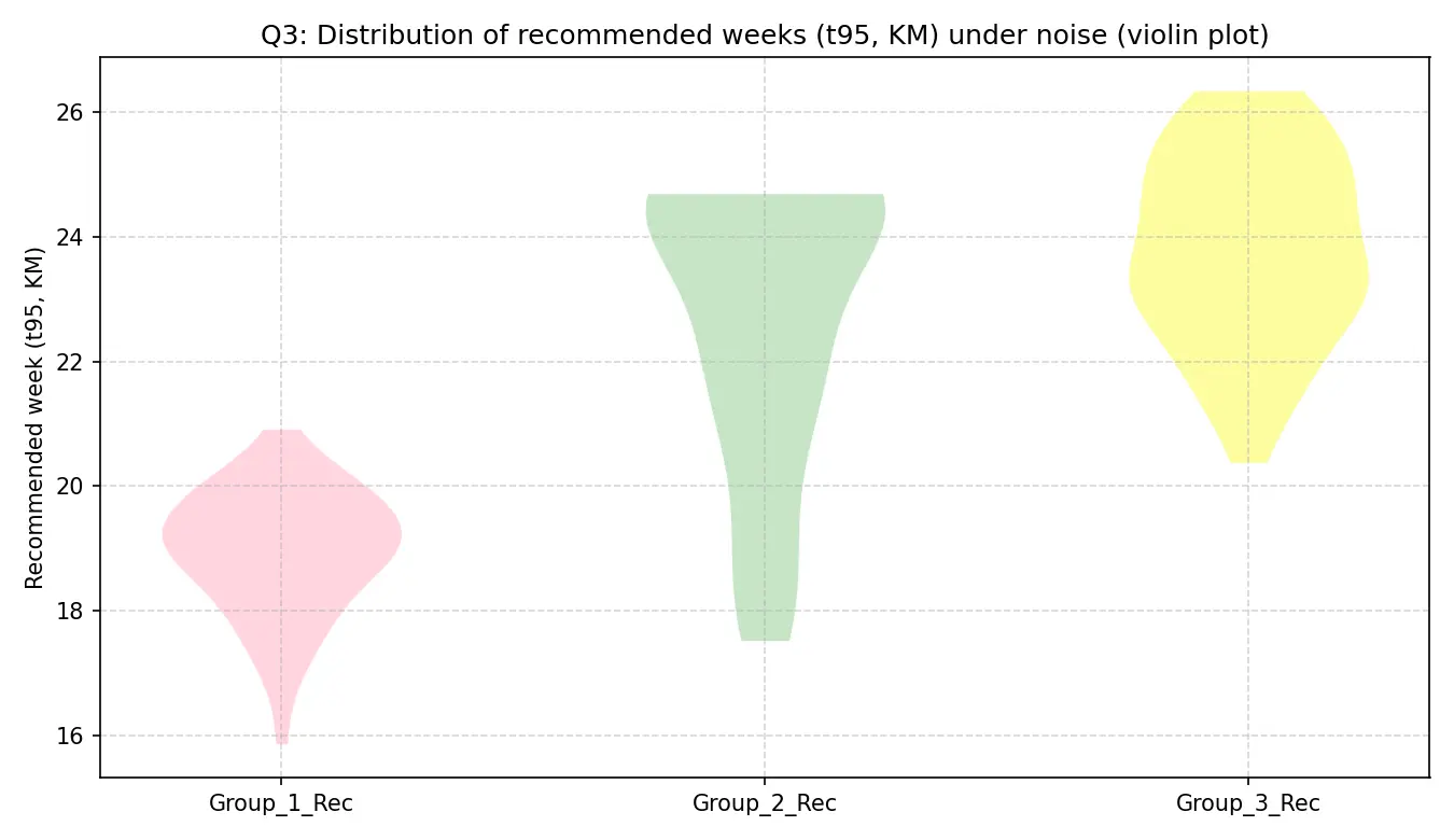
噪声实验下的小提琴图
该过程等价于研究映射
Φ : { y i j } ↦ ( C , t 1 , p , … , t K , p ) \Phi:\ \{y_{ij}\} \mapsto (\mathcal{C},\; t_{1,p},\dots,t_{K,p})
Φ : { y ij } ↦ ( C , t 1 , p , … , t K , p )
在加噪扰动下的分布。若映射对噪声敏感,则输出分布会显示大方差或多峰性。实验结果如图11 。
图中每个切点的小提琴形状都非常狭窄,且集中在一个很小的BMI值范围内。每个风险组对应的推荐孕周同样呈现出非常集中的分布。这说明基于本文分箱模型的BMI切点和临床建议(即对不同风险的个体建议不同的复查时间)都非常稳定。这强力证明了本文找到的BMI阈值是数据内在的、稳定的结构性特征,对噪声具有高度的鲁棒性。
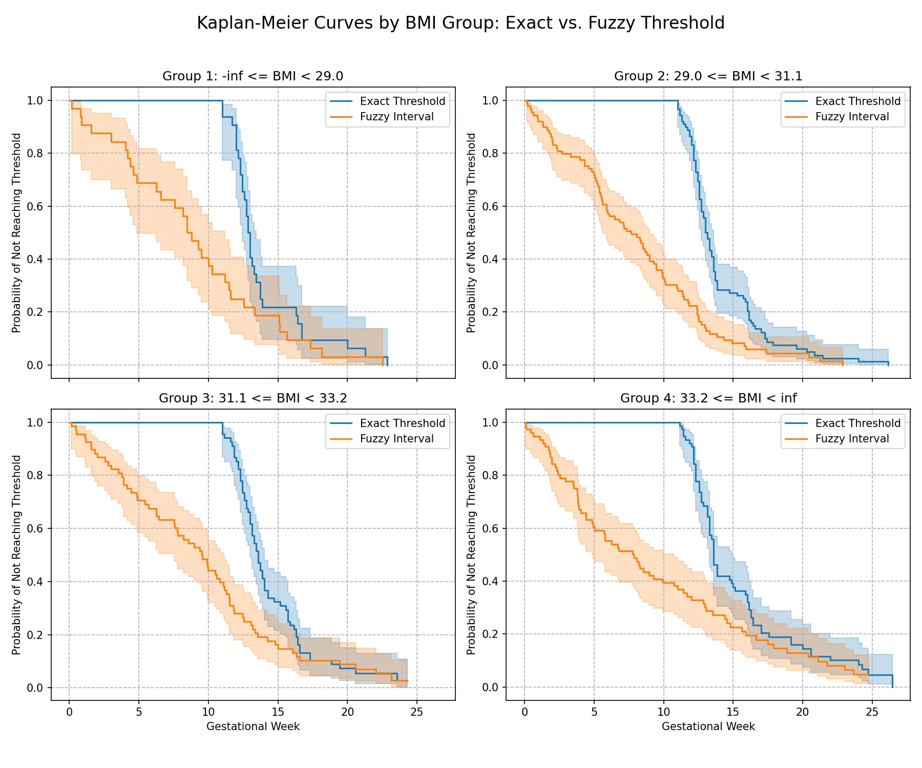
然后是模糊阈值实验。给定模糊阈值区间 [ 0.039 , 0.041 ] [0.039,0.041] [ 0.039 , 0.041 ]
1.若存在最早的 j j j y i j > c u y_{ij} > c_u y ij > c u R i = w i j R_i=w_{ij} R i = w ij L i L_i L i R i R_i R i y i j > c u y_{ij} > c_u y ij > c u L i = max j w i j L_i=\max_j w_{ij} L i = max j w ij
与精确阈值判定不同,模糊阈值把只有超过上界 c u c_u c u ( c ℓ , c u ] (c_\ell,c_u] ( c ℓ , c u ]
对区间样本采用一次均匀插补:
T i f u z z y ∼ U n i f ( L i , R i ) . T_i^{\mathrm{fuzzy}} \sim \mathrm{Unif}(L_i,R_i).
T i fuzzy ∼ Unif ( L i , R i ) .
然后在已给定的 BMI 分箱下分别计算两种规则(精确阈值 vs. 模糊阈值)得到的组内 KM 估计与第 p p p t g , p exact t_{g,p}^{\text{exact}} t g , p exact t g , p fuzzy t_{g,p}^{\text{fuzzy}} t g , p fuzzy
不同风险组的模糊阈值与精确阈值对比结果如图所示。据图分析,即使在考虑了测量误差的更苛刻条件下,不同风险组之间的差异依然显著。且组内 KM 估计与第 p p p t g , p exact t_{g,p}^{\text{exact}} t g , p exact t g , p fuzzy t_{g,p}^{\text{fuzzy}} t g , p fuzzy
问题三的模型的建立和求解
根据问题二对原始BMI分组的探究,可知原始分组在本题也不是最优解。由于原始数据中大量的左删失情况,MI+Cox的解决方法效果并不理想,因此本文使用了在高删失下更稳定地估计高分位的AFT模型,另外AFT和半参数的Cox一样支持BMI、年龄、IVF等协变量,符合问题三中要考虑多因素影响的要求。
模型建立
为了将 BMI 连续变量分割为 k k k D = { ( x i , y i ) } i = 1 n \mathcal{D}=\{(x_i,y_i)\}_{i=1}^n D = {( x i , y i ) } i = 1 n x i ∈ R x_i\in\mathbb{R} x i ∈ R i i i y i ∈ R y_i\in\mathbb{R} y i ∈ R π 25 = P ( T ≤ 25 ) \pi_{25}=P(T\le 25) π 25 = P ( T ≤ 25 ) t 95 t_{95} t 95 T T T
区间删失数据处理
对个体 i i i { t i , 1 , … , t i , m i } \{t_{i,1},\ldots,t_{i,m_i}\} { t i , 1 , … , t i , m i } { y i , 1 , … , y i , m i } \{y_{i,1},\ldots,y_{i,m_i}\} { y i , 1 , … , y i , m i } τ = 0.04 \tau=0.04 τ = 0.04 [ L i , R i ] [L_i,R_i] [ L i , R i ]
[ L i , R i ] = { [ 0 , t i , j ∗ ] , 左删失: y i , 1 ≥ τ , [ t i , j ∗ − 1 , t i , j ∗ ] , 区间删失: ∃ j ∗ s.t. y i , j ∗ − 1 < τ ≤ y i , j ∗ , [ t i , m i , + ∞ ) , 右删失: ∀ j , y i , j < τ . [L_i,R_i]=
\begin{cases}
[0,t_{i,j^\ast}], & \text{左删失:} y_{i,1}\ge \tau,\\
[t_{i,j^\ast-1},t_{i,j^\ast}], & \text{区间删失:}\exists j^\ast \text{ s.t. } y_{i,j^\ast-1}<\tau\le y_{i,j^\ast},\\
[t_{i,m_i},+\infty), & \text{右删失:}\forall j,\;y_{i,j}<\tau.
\end{cases}
[ L i , R i ] = ⎩ ⎨ ⎧ [ 0 , t i , j ∗ ] , [ t i , j ∗ − 1 , t i , j ∗ ] , [ t i , m i , + ∞ ) , 左删失: y i , 1 ≥ τ , 区间删失: ∃ j ∗ s.t. y i , j ∗ − 1 < τ ≤ y i , j ∗ , 右删失: ∀ j , y i , j < τ .
定义删失类型指示 ( δ i left , δ i int , δ i right ) ∈ { 0 , 1 } 3 (\delta_i^{\text{left}},\delta_i^{\text{int}},\delta_i^{\text{right}})\in\{0,1\}^3 ( δ i left , δ i int , δ i right ) ∈ { 0 , 1 } 3
区间删失对统计推断的含义
左删失仅给出 T i ≤ R i T_i\le R_i T i ≤ R i T i > L i T_i> L_i T i > L i L i < T i ≤ R i L_i<T_i\le R_i L i < T i ≤ R i
在参数模型中,这三类观测贡献不同的似然项;在非参 KM 框架中,需先通过“条件抽样”将其转化为仅含右删失的样本以便估计阶梯生存曲线。
AFT 加速失效时间模型
AFT 模型刻画 log T \log T log T
log T i = x i ⊤ β + σ ϵ i , ϵ i ∼ i.i.d. F 0 , \log T_i=\mathbf{x}_i^\top\boldsymbol{\beta}+\sigma\epsilon_i,\qquad \epsilon_i\overset{\text{i.i.d.}}{\sim}F_0,
log T i = x i ⊤ β + σ ϵ i , ϵ i ∼ i.i.d. F 0 ,
其中 x i \mathbf{x}_i x i F 0 F_0 F 0
μ i ≡ x i ⊤ β , F i ( t ) ≡ P ( T i ≤ t ∣ x i ) = F 0 ( log t − μ i σ ) , S i ( t ) = 1 − F i ( t ) . \mu_i\equiv\mathbf{x}_i^\top\boldsymbol{\beta},\quad
F_i(t)\equiv P(T_i\le t\mid \mathbf{x}_i)=F_0\!\left(\frac{\log t-\mu_i}{\sigma}\right),\quad
S_i(t)=1-F_i(t).
μ i ≡ x i ⊤ β , F i ( t ) ≡ P ( T i ≤ t ∣ x i ) = F 0 ( σ log t − μ i ) , S i ( t ) = 1 − F i ( t ) .
log-normal:F 0 = Φ F_0=\Phi F 0 = Φ t p = exp { μ i + σ Φ − 1 ( p ) } t_p=\exp\{\mu_i+\sigma \Phi^{-1}(p)\} t p = exp { μ i + σ Φ − 1 ( p )} S i ( t ) = 1 − Φ ( ( log t − μ i ) / σ ) S_i(t)=1-\Phi\big((\log t-\mu_i)/\sigma\big) S i ( t ) = 1 − Φ ( ( log t − μ i ) / σ ) k = 1 / σ k=1/\sigma k = 1/ σ λ = exp ( μ i ) \lambda=\exp(\mu_i) λ = exp ( μ i ) F i ( t ) = 1 − exp { − ( t / λ ) k } F_i(t)=1-\exp\{-(t/\lambda)^k\} F i ( t ) = 1 − exp { − ( t / λ ) k } F i ( t ) = [ 1 + ( t / λ ) − k ] − 1 F_i(t)=\big[1+\big(t/\lambda\big)^{-k}\big]^{-1} F i ( t ) = [ 1 + ( t / λ ) − k ] − 1
区间删失 AFT 似然: F 0 , f 0 F_0,f_0 F 0 , f 0 i i i
ℓ i ( β , σ ) = { log F i ( R i ) , δ i left = 1 , log { F i ( R i ) − F i ( L i ) } , δ i int = 1 , log { 1 − F i ( L i ) } , δ i right = 1 , \ell_i(\boldsymbol{\beta},\sigma)=
\begin{cases}
\log F_i(R_i),& \delta_i^{\text{left}}=1,\\
\log\big\{F_i(R_i)-F_i(L_i)\big\},& \delta_i^{\text{int}}=1,\\
\log\big\{1-F_i(L_i)\big\},& \delta_i^{\text{right}}=1,
\end{cases}
ℓ i ( β , σ ) = ⎩ ⎨ ⎧ log F i ( R i ) , log { F i ( R i ) − F i ( L i ) } , log { 1 − F i ( L i ) } , δ i left = 1 , δ i int = 1 , δ i right = 1 ,
总体对数似然 ℓ = ∑ i ℓ i \ell=\sum_i \ell_i ℓ = ∑ i ℓ i ( β ^ , σ ^ ) (\hat{\boldsymbol{\beta}},\hat{\sigma}) ( β ^ , σ ^ ) 2 k − 2 ℓ ( θ ^ ) 2k-2\ell(\hat{\theta}) 2 k − 2 ℓ ( θ ^ ) k k k
个体层预测量:
分位时间:t 90 , t 95 t_{90},t_{95} t 90 , t 95 t p = inf { t : F i ( t ) ≥ p } t_p=\inf\{t:F_i(t)\ge p\} t p = inf { t : F i ( t ) ≥ p } t p = exp { μ i + σ Φ − 1 ( p ) } t_p=\exp\{\mu_i+\sigma \Phi^{-1}(p)\} t p = exp { μ i + σ Φ − 1 ( p )} π 25 , i = P ( T i ≤ 25 ) = F i ( 25 ) \pi_{25,i}=P(T_i\le 25)=F_i(25) π 25 , i = P ( T i ≤ 25 ) = F i ( 25 ) π 25 \pi_{25} π 25 t 95 t_{95} t 95
基于 AFT 拟合结果的 MI 条件插补
令 F i F_i F i M M M
T i ( m ) ∼ { F i − 1 ( U ⋅ F i ( R i ) ) , 左删失 ( 0 , R i ] , F i − 1 ( F i ( L i ) + U ⋅ ( F i ( R i ) − F i ( L i ) ) ) , 区间删失 ( L i , R i ] , U ∼ Unif ( 0 , 1 ) . T_i^{(m)}\sim
\begin{cases}
F_i^{-1}\!\big(U\cdot F_i(R_i)\big), & \text{左删失 } (0,R_i],\\
F_i^{-1}\!\big(F_i(L_i)+U\cdot(F_i(R_i)-F_i(L_i))\big), & \text{区间删失 } (L_i,R_i],
\end{cases}
\quad U\sim \text{Unif}(0,1).
T i ( m ) ∼ { F i − 1 ( U ⋅ F i ( R i ) ) , F i − 1 ( F i ( L i ) + U ⋅ ( F i ( R i ) − F i ( L i )) ) , 左删失 ( 0 , R i ] , 区间删失 ( L i , R i ] , U ∼ Unif ( 0 , 1 ) .
右删失保持不变(仅记录删失界与删失指示)。每次插补得到仅含右删失的样本,之后据此计算 KM 曲线与分位数。本文取 M = 200 M=200 M = 200
监督式分箱(回归树)(SSE 准则)
给定分组数 K K K MIN_LEAF \text{MIN\_LEAF} MIN_LEAF C = { c 1 < ⋯ < c K − 1 } \mathcal{C}=\{c_1<\cdots<c_{K-1}\} C = { c 1 < ⋯ < c K − 1 }
min C ∑ g = 1 K ∑ i ∈ I g ( C ) ( y i − y ˉ g ) 2 , y ˉ g = 1 ∣ I g ∣ ∑ i ∈ I g y i . \min_{\mathcal{C}}\; \sum_{g=1}^K \sum_{i\in \mathcal{I}_g(\mathcal{C})}\big(y_i-\bar{y}_g\big)^2,
\quad \bar{y}_g=\frac{1}{|\mathcal{I}_g|}\sum_{i\in \mathcal{I}_g} y_i.
C min g = 1 ∑ K i ∈ I g ( C ) ∑ ( y i − y ˉ g ) 2 , y ˉ g = ∣ I g ∣ 1 i ∈ I g ∑ y i .
使用贪心策略:从全集出发,枚举可行切点,以降幅
Δ SSE = SSE parent − SSE left − SSE right \Delta \text{SSE}=\text{SSE}_{\text{parent}}-\text{SSE}_{\text{left}}-\text{SSE}_{\text{right}}
Δ SSE = SSE parent − SSE left − SSE right
最大者为优,直至达到 K K K Δ SSE < MIN_GAIN \Delta \text{SSE}<\text{MIN\_GAIN} Δ SSE < MIN_GAIN y i = π 25 , i y_i=\pi_{25,i} y i = π 25 , i K = 3 , MIN_LEAF = 30 K=3,\ \text{MIN\_LEAF}=30 K = 3 , MIN_LEAF = 30
KM 估计与多重合并
对第 m m m { ( T i ( m ) , δ i ( m ) ) } \{(T_i^{(m)},\delta_i^{(m)})\} {( T i ( m ) , δ i ( m ) )} { t j } \{t_j\} { t j }
S ^ ( m ) ( t ) = ∏ t j ≤ t ( 1 − d j ( m ) n j ( m ) ) , \widehat{S}^{(m)}(t)=\prod_{t_j\le t}\left(1-\frac{d_j^{(m)}}{n_j^{(m)}}\right),
S ( m ) ( t ) = t j ≤ t ∏ ( 1 − n j ( m ) d j ( m ) ) ,
其中 d j ( m ) d_j^{(m)} d j ( m ) t j t_j t j n j ( m ) n_j^{(m)} n j ( m )
S ^ ( t ) = median { S ^ ( 1 ) ( t ) , … , S ^ ( M ) ( t ) } , \widehat{S}(t)=\operatorname{median}\big\{\widehat{S}^{(1)}(t),\ldots,\widehat{S}^{(M)}(t)\big\},
S ( t ) = median { S ( 1 ) ( t ) , … , S ( M ) ( t ) } ,
并记录 25–75% 分位带作为不确定性区间。
分位数与推荐时点
KM 分位数取
t ^ α KM = inf { t : S ^ ( t ) ≤ α } , \hat{t}_\alpha^{\text{KM}}=\inf\{t:\widehat{S}(t)\le \alpha\},
t ^ α KM = inf { t : S ( t ) ≤ α } ,
AFT 分位数取个体分位的组内中位。对第 k k k
y k = { round ( median { t ^ 0.05 KM , ( m ) } m = 1 M / 0.5 ) × 0.5 , KM 可用 ; round ( median { t ^ 0.05 AFT } / 0.5 ) × 0.5 , 否则 , y_k=
\begin{cases}
\text{round}\Big(\operatorname{median}\{\hat{t}_{0.05}^{\text{KM},(m)}\}_{m=1}^M/0.5\Big)\times 0.5,& \text{KM 可用};\\[2pt]
\text{round}\Big(\operatorname{median}\{\hat{t}_{0.05}^{\text{AFT}}\}/0.5\Big)\times 0.5,& \text{否则},
\end{cases}
y k = ⎩ ⎨ ⎧ round ( median { t ^ 0.05 KM , ( m ) } m = 1 M /0.5 ) × 0.5 , round ( median { t ^ 0.05 AFT } /0.5 ) × 0.5 , KM 可用 ; 否则 ,
其中 round 表示四舍五入到 0.5 周。该规则保证 P ( T > y k ) ≈ 0.05 P(T>y_k)\approx 0.05 P ( T > y k ) ≈ 0.05
模型求解
本节给出似然构造、参数估计、分布选择、监督分箱、MI+KM 合并、KM–AFT 对齐度与推荐生成的完整实现细节与数值结果。
区间删失 AFT 的极大似然与分布选择
以log-normal / Weibull / log-logistic为候选,采用R语言中的\texttt{survreg}做interval-censor生存回归,在 Surv ( L i , R i , type=''interval2'' ) \text{Surv}(L_i,R_i,\texttt{type=''interval2''}) Surv ( L i , R i , type=’’interval2’’ ) μ ^ i = x i ⊤ β ^ \hat{\mu}_i=\mathbf{x}_i^\top\hat{\boldsymbol{\beta}} μ ^ i = x i ⊤ β ^ σ ^ \hat{\sigma} σ ^ t 90 , t 95 t_{90},t_{95} t 90 , t 95 π 25 = F i ( 25 ) \pi_{25}=F_i(25) π 25 = F i ( 25 )
固定时点达标概率:
π 25 , i = P ( T i ≤ 25 ) = Φ ( ( log 25 − μ ^ i ) / σ ^ ) , \pi_{25,i}=P(T_i\le 25)=\Phi\big((\log 25-\hat{\mu}_i)/\hat{\sigma}\big),
π 25 , i = P ( T i ≤ 25 ) = Φ ( ( log 25 − μ ^ i ) / σ ^ ) ,
是监督分箱的首选目标(USE_METRIC=‘‘pi_25’’),能更直接反映“到 25 周是否已达标”的风险梯度。
监督式分箱的求解与性质
切点搜索:排序 BMI 后仅在相邻样本中点处枚举切点,时间复杂度 O ( n ) O(n) O ( n ) O ( n K ) O(nK) O ( n K ) ≥ MIN_LEAF \ge \text{MIN\_LEAF} ≥ MIN_LEAF Δ SSE < MIN_GAIN \Delta\text{SSE}<\text{MIN\_GAIN} Δ SSE < MIN_GAIN
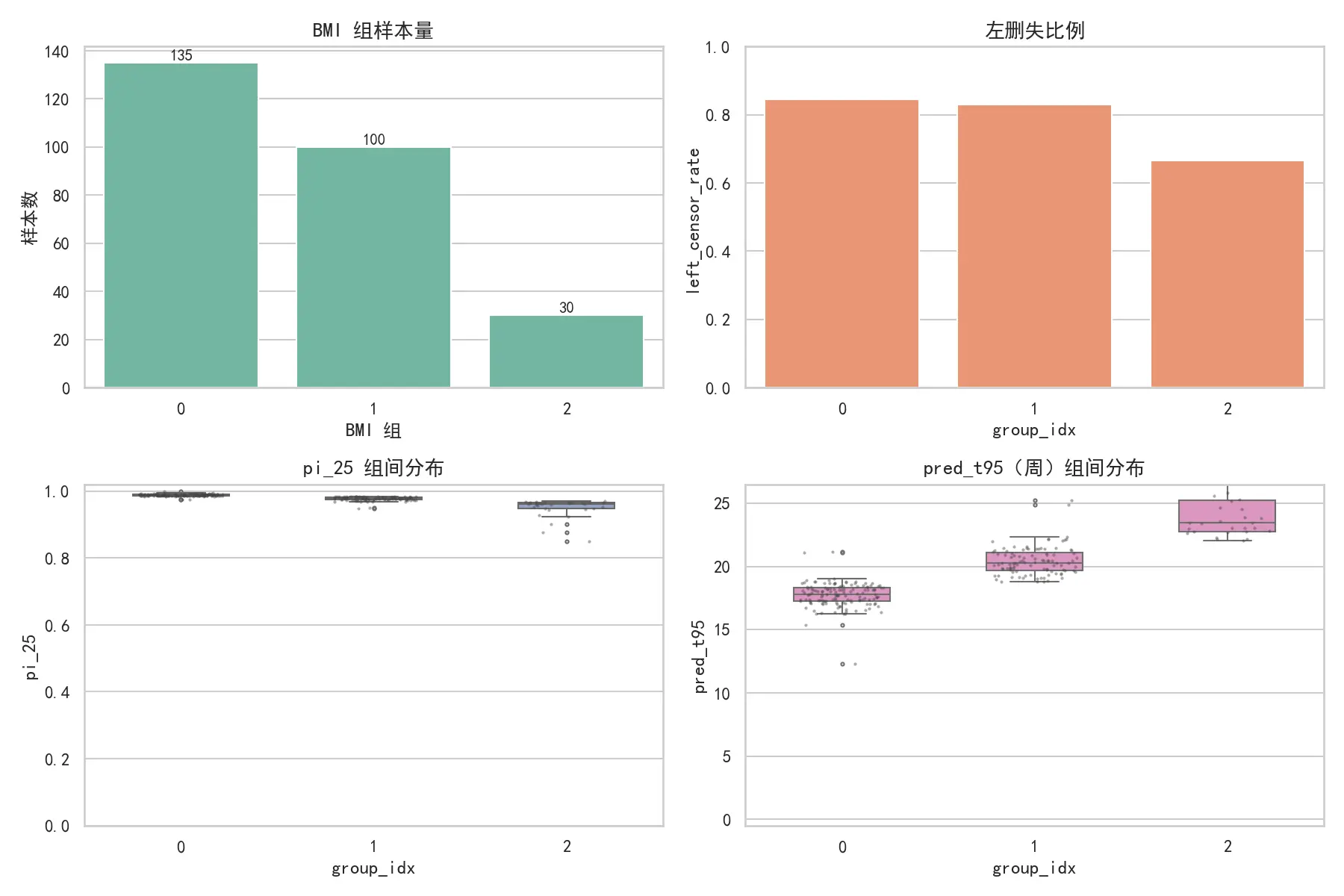
组别编号 BMI范围
0
[ 20.70 , 31.73 ] [20.70,\,31.73] [ 20.70 , 31.73 ]
1
[ 31.75 , 35.63 ] [31.75,\,35.63] [ 31.75 , 35.63 ]
2
[ 35.67 , 46.88 ] [35.67,\,46.88] [ 35.67 , 46.88 ]
MI 条件插补与 KM 合并的实现
对每个左/区间删失样本,按个体 F i F_i F i M = 200 M=200 M = 200 t ∈ [ 0 , 26 ] t\in[0,26] t ∈ [ 0 , 26 ] S ^ ( t ) \widehat{S}(t) S ( t ) t 95 t_{95} t 95 t 95 t_{95} t 95
KM 分位时间估计结果:
组别 t 95 t_{95} t 95 t 95 t_{95} t 95 t 95 t_{95} t 95 t 90 t_{90} t 90 t 90 t_{90} t 90 t 90 t_{90} t 90
0
17.520
17.049
18.218
14.456
14.114
14.836
1
/
/
/
17.675
17.177
18.145
2
/
/
/
/
/
/
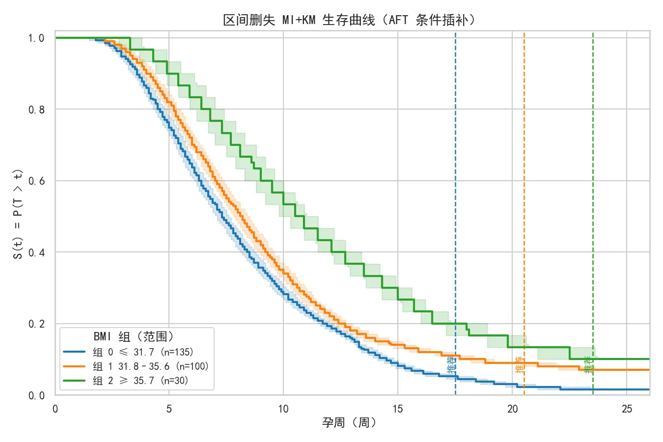
组别编号
BMI值范围
推荐最佳检测点
0
31.7及以下
17.5周
1
[ 31.7 , 35.7 ) [31.7,35.7) [ 31.7 , 35.7 ) 20.5周
2
35.7及以上
23.5周
模型评估
目标单调性与对数秩检验
分组配对的对数秩检验(合并 p 值)
配对组 卡方值 自由度 合并p值 统计量均值 样本数
0 vs 1
585.307
400
3.948 × 10 − 9 3.948\times 10^{-9} 3.948 × 1 0 − 9 1.511
200
1 vs 2
824.746
400
1.096 × 10 − 31 1.096\times 10^{-31} 1.096 × 1 0 − 31 2.369
200
目标的单调性强(Spearman( BMI , pred_t95 ) = 0.953 (\text{BMI},\ \text{pred\_t95})=0.953 ( BMI , pred_t95 ) = 0.953 3.95 × 10 − 9 3.95\times 10^{-9} 3.95 × 1 0 − 9 1.10 × 10 − 31 1.10\times 10^{-31} 1.10 × 1 0 − 31
KM–AFT 对齐度的定义与计算
在诊断窗 [ 8 , 24 ] [8,24] [ 8 , 24 ] S ~ KM ( t ) \widetilde{S}^{\text{KM}}(t) S KM ( t ) S ~ AFT ( t ) \widetilde{S}^{\text{AFT}}(t) S AFT ( t )
align_L1 8 – 24 = 1 ∣ G ∣ ∑ t ∈ G ∣ S ~ KM ( t ) − S ~ AFT ( t ) ∣ , align_sup 8 – 24 = max t ∈ G ∣ S ~ KM ( t ) − S ~ AFT ( t ) ∣ , \text{align\_L1}_{8\text{--}24}
=\frac{1}{|G|}\sum_{t\in G}\big|\widetilde{S}^{\text{KM}}(t)-\widetilde{S}^{\text{AFT}}(t)\big|,\quad
\text{align\_sup}_{8\text{--}24}
=\max_{t\in G}\big|\widetilde{S}^{\text{KM}}(t)-\widetilde{S}^{\text{AFT}}(t)\big|,
align_L1 8 – 24 = ∣ G ∣ 1 t ∈ G ∑ S KM ( t ) − S AFT ( t ) , align_sup 8 – 24 = t ∈ G max S KM ( t ) − S AFT ( t ) ,
其中 G = { 8 , 8.1 , … , 24 } G=\{8,8{.}1,\ldots,24\} G = { 8 , 8 . 1 , … , 24 } 0.1 0.1 0.1
计算结果:
组0:L1 0.00617,sup 0.01898(优秀)
组1:L1 0.02591,sup 0.04716(良好)
组2:L1 0.06069,sup 0.09140(一般,由于样本小且左删失严重)
敏感性分析
为了验证模型结果的稳定性,项目进行了敏感性分析,通过向原始数据注入随机噪声并重复建模过程,观察关键结果(BMI切分点和推荐孕周)的变动情况。
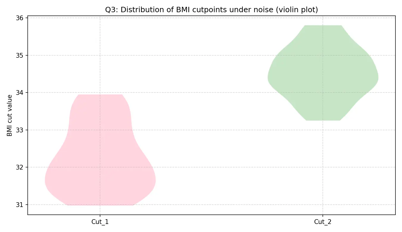
噪声实验下的分布小提琴图
左图展示了在数据有噪声的情况下,两个BMI切分点的分布。可以看出,第一个切分点(粉色)非常稳定,集中在31-34之间;第二个切分点(绿色)波动稍大,但仍稳定在33-36之间。这证明了BMI分组方式是稳健的。
右图展示了各组推荐孕周的分布。可以看出,低BMI组的推荐时间非常稳定(小提琴很“瘦”),而高BMI组的推荐时间不确定性更大(小提琴更“胖”),这与高BMI组样本量少、删失率高的现实情况相符。尽管如此,各组的推荐时间核心区间清晰可辨,证明了最终推荐策略的整体可靠性。
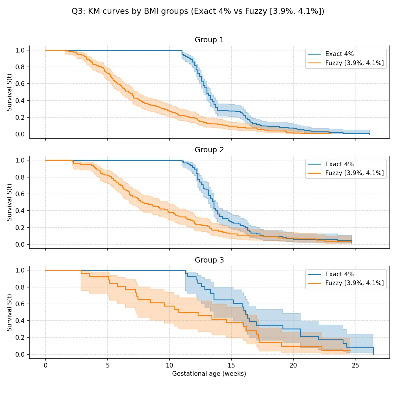
此外,针对这三个不同的BMI分组,绘制出KM生存曲线,验证其敏感性。
从图中可以看出,在所有三个组中,橙色曲线(模糊定义)都位于蓝色曲线(精确定义)的下方,这意味着在模糊定义下,达标时间似乎发生得更早。然而,两条曲线的整体形状、趋势以及置信区间的大部分是重叠的,表明虽然定义不同会导致数值上的轻微差异,但并不会从根本上改变“BMI越高,达标时间越晚”这一核心结论。
问题四的模型的建立和求解
该题的核心任务是为女胎建立一个准确的异常判定方法。与男胎不同,女胎不携带Y染色体,因此无法使用Y染色体浓度作为直接的判断依据。因此,必须综合利用其他多种生物信息学指标,如各关键染色体(13, 18, 21, X)的Z值、GC含量、测序读段数以及孕妇的BMI等个人信息,来构建一个高精度的分类模型,以判断胎儿是否存在21、18或13号染色体的非整倍体异常。
模型建立
考虑到临床应用的严肃性,模型的评估不能仅仅依赖于传统的准确率。在产前检测中,假阴性,即未能检测出实际异常的胎儿,会带来严重的临床后果而错过干预窗口,其代价远高于假阳性,即错误地将正常胎儿标记为异常。因此,本文采纳了更符合临床需求的非对称代价函数作为模型优化的最终目标。
特征工程
在将数据输入模型之前,本文执行了一系列特征工程步骤,以增强原始数据的表达能力并满足模型要求。这些步骤包括:
(1)**缺失值处理:**部分样本的“孕妇BMI”特征存在缺失值。本文采用中位数插补的方法来填充这些缺失值,以保证数据的完整性。
(2)数据清洗 :对数据进行了清洗,并根据文献以及临床经验设定了一个质量控制标准。本文仅在X染色体Z值的绝对值小于2.5的“高置信度”样本上进行后续所有操作。这一步骤排除了14个信号可能不可靠的样本,旨在构建一个在常规情况下更稳定、更可靠的模型。
(3)**交互特征构建:**为了捕捉关键变量之间可能存在的非线性协同效应,本文构建了新的交互特征。具体而言,将各染色体的Z值与X染色体浓度相乘:
z s c o r e c h r f f = z s c o r e c h r × x c o n c e n t r a t i o n , where c h r ∈ { 13 , 18 , 21 } , z_score_chr_ff = z_score_chr \times x_concentration, \quad \text{where } chr \in \{13, 18, 21\} ,
z s cor e c h r f f = z s cor e c h r × x c o n ce n t r a t i o n , where c h r ∈ { 13 , 18 , 21 } ,
这些交互特征旨在放大在高胎儿浓度下Z值的信号。
(4)**特征离散化:**观察到X染色体的Z值的绝对值在特定区间有不同的临床意义,因此对其进行分箱处理,将其转化为一个分类特征:
1.区间: [ 0 , 2.5 ) , [ 2.5 , 3 ) , [ 3 , + ∞ ) [0, 2.5), [2.5, 3), [3, +∞) [ 0 , 2.5 ) , [ 2.5 , 3 ) , [ 3 , + ∞ )
2.标签: 正常(ZX), 临界(ZX), 异常(ZX)
(5)**特征缩放:**由于支持向量机(SVM)对特征的尺度非常敏感,在将其输入SVM模型之前,对所有数值型特征进行了标准化处理,将每个特征j j j
x i j ′ = x i j − μ j σ j x'_{ij} = \frac{x_{ij} - \mu_j}{\sigma_j}
x ij ′ = σ j x ij − μ j
其中,μ j \mu_j μ j σ j \sigma_j σ j j j j
(6)**最终特征列表:**经过上述所有处理步骤后,最终输入到模型中的完整特征列表是:年龄,孕周,BMI,比对率,重复率,唯一比对读段数,GC 含量,13 号染色体 Z 分数,18 号染色体Z值 ,21 号染色体Z值,X染色体Z值,X染色体浓度,21 号染色体Z值与胎儿 DNA 含量的交互特征,18 号染色体Z值与胎儿DNA含量的交互特征,13号染色体Z值与胎儿DNA含量的交互特征,X 染色体 Z 值分箱后为正常(ZX) 的独热编码特征,X 染色体 Z 值分箱后为临界(ZX) 的独热编码特征,X 染色体 Z值分箱后为异常(ZX) 的独热编码特征。
支持向量机(SVM)
SVM的核心思想是在特征空间中寻找一个能将不同类别样本最大程度分开的最优超平面。对于给定的训练数据集 D = { ( x i , y i ) } i = 1 N D = \{(x_i, y_i)\}_{i=1}^N D = {( x i , y i ) } i = 1 N x i ∈ R p x_i \in \mathbb{R}^p x i ∈ R p y i ∈ { − 1 , 1 } y_i \in \{-1, 1\} y i ∈ { − 1 , 1 }
min w , b , ξ 1 2 ∥ w ∥ 2 + C ∑ i = 1 N ξ i , \min_{w, b, \xi} \frac{1}{2} \|w\|^2 + C \sum_{i=1}^N \xi_i ,
w , b , ξ min 2 1 ∥ w ∥ 2 + C i = 1 ∑ N ξ i ,
约束条件为:
y i ( w T x i + b ) ≥ 1 − ξ i , ∀ i = 1 , … , N , ξ i ≥ 0 , ∀ i = 1 , … , N , y_i(w^T x_i + b) \ge 1 - \xi_i, \quad \forall i=1, \dots, N ,
\xi_i \ge 0, \quad \forall i=1, \dots, N ,
y i ( w T x i + b ) ≥ 1 − ξ i , ∀ i = 1 , … , N , ξ i ≥ 0 , ∀ i = 1 , … , N ,
其中,w ∈ R p w \in \mathbb{R}^p w ∈ R p b ∈ R b \in \mathbb{R} b ∈ R ∥ w ∥ 2 \|w\|^2 ∥ w ∥ 2 C > 0 C > 0 C > 0 ξ i \xi_i ξ i
接着,为了处理非线性可分的数据,SVM使用核技巧 将原始特征空间映射到一个更高维的希尔伯特空间:H \mathcal{H} H ϕ : R p → H \phi: \mathbb{R}^p \to \mathcal{H} ϕ : R p → H K ( x i , x j ) = ⟨ ϕ ( x i ) , ϕ ( x j ) ⟩ K(x_i, x_j) = \langle \phi(x_i), \phi(x_j) \rangle K ( x i , x j ) = ⟨ ϕ ( x i ) , ϕ ( x j )⟩ ϕ ( x ) \phi(x) ϕ ( x )
在本项目中,本文选用了高斯核(RBF核),其定义如下:
K ( x i , x j ) = exp ( − γ ∥ x i − x j ∥ 2 ) K(x_i, x_j) = \exp(-\gamma \|x_i - x_j\|^2)
K ( x i , x j ) = exp ( − γ ∥ x i − x j ∥ 2 )
其中,γ > 0 \gamma > 0 γ > 0 γ \gamma γ
通过求解原始问题的对偶问题(Dual Problem),得到最终的决策函数:
f ( x ) = sgn ( ∑ i = 1 N α i y i K ( x i , x ) + b ) f(x) = \text{sgn} \left( \sum_{i=1}^N \alpha_i y_i K(x_i, x) + b \right)
f ( x ) = sgn ( i = 1 ∑ N α i y i K ( x i , x ) + b )
其中,α i \alpha_i α i α i \alpha_i α i
极端梯度提升(XGBoost)
XGBoost是一种基于梯度提升决策树算法的高效、可扩展的实现。其构建的是一个由 K K K x i x_i x i y ^ i \hat{y}_i y ^ i
y ^ i = ∑ k = 1 K f k ( x i ) , f k ∈ F \hat{y}_i = \sum_{k=1}^K f_k(x_i), \quad f_k \in \mathcal{F}
y ^ i = k = 1 ∑ K f k ( x i ) , f k ∈ F
其中 F \mathcal{F} F
模型通过最小化一个包含损失函数和正则化项的目标函数来进行训练:
Obj = ∑ i = 1 N l ( y i , y ^ i ) + ∑ k = 1 K Ω ( f k ) , \text{Obj} = \sum_{i=1}^N l(y_i, \hat{y}_i) + \sum_{k=1}^K \Omega(f_k),
Obj = i = 1 ∑ N l ( y i , y ^ i ) + k = 1 ∑ K Ω ( f k ) ,
其中,l ( y i , y ^ i ) l(y_i, \hat{y}_i) l ( y i , y ^ i )
l ( y i , y ^ i ) = − [ y i log ( p i ) + ( 1 − y i ) log ( 1 − p i ) ] l(y_i, \hat{y}_i) = -[y_i \log(p_i) + (1-y_i) \log(1-p_i)]
l ( y i , y ^ i ) = − [ y i log ( p i ) + ( 1 − y i ) log ( 1 − p i )]
其中 p i = σ ( y ^ i ) p_i = \sigma(\hat{y}_i) p i = σ ( y ^ i ) σ \sigma σ Ω ( f ) \Omega(f) Ω ( f )
Ω ( f ) = γ T + 1 2 λ ∑ j = 1 T w j 2 \Omega(f) = \gamma T + \frac{1}{2} \lambda \sum_{j=1}^T w_j^2
Ω ( f ) = γ T + 2 1 λ j = 1 ∑ T w j 2
T T T w j w_j w j j j j γ \gamma γ λ \lambda λ
由于模型是分步迭代训练的,在第 t t t f t f_t f t
Obj ( t ) = ∑ i = 1 N l ( y i , y ^ i ( t − 1 ) + f t ( x i ) ) + Ω ( f t ) \text{Obj}^{(t)} = \sum_{i=1}^N l(y_i, \hat{y}_i^{(t-1)} + f_t(x_i)) + \Omega(f_t)
Obj ( t ) = i = 1 ∑ N l ( y i , y ^ i ( t − 1 ) + f t ( x i )) + Ω ( f t )
通过对损失函数进行二阶泰勒展开,可以近似得到在第 t t t
Obj ( t ) ≈ ∑ i = 1 N [ l ( y i , y ^ i ( t − 1 ) ) + g i f t ( x i ) + 1 2 h i f t ( x i ) 2 ] + Ω ( f t ) \text{Obj}^{(t)} \approx \sum_{i=1}^N [l(y_i, \hat{y}_i^{(t-1)}) + g_i f_t(x_i) + \frac{1}{2} h_i f_t(x_i)^2] + \Omega(f_t)
Obj ( t ) ≈ i = 1 ∑ N [ l ( y i , y ^ i ( t − 1 ) ) + g i f t ( x i ) + 2 1 h i f t ( x i ) 2 ] + Ω ( f t )
其中 g i g_i g i h i h_i h i y ^ i ( t − 1 ) \hat{y}_i^{(t-1)} y ^ i ( t − 1 )
模型集成与代价优化
本文将两个基模型的概率输出进行线性加权平均,以得到最终的集成概率:
P ensemble ( x ) = w ⋅ P XGB ( x ) + ( 1 − w ) ⋅ P SVM ( x ) , P_{\text{ensemble}}(x) = w \cdot P_{\text{XGB}}(x) + (1-w) \cdot P_{\text{SVM}}(x) ,
P ensemble ( x ) = w ⋅ P XGB ( x ) + ( 1 − w ) ⋅ P SVM ( x ) ,
其中,P XGB ( x ) P_{\text{XGB}}(x) P XGB ( x ) P SVM ( x ) P_{\text{SVM}}(x) P SVM ( x ) x x x w ∈ [ 0 , 1 ] w \in [0, 1] w ∈ [ 0 , 1 ]
基于集成概率,本文使用一个分类阈值 τ \tau τ
y ^ = { 1 if P ensemble ( x ) > τ 0 otherwise \hat{y} = \begin{cases} 1 & \text{if } P_{\text{ensemble}}(x) > \tau \\ 0 & \text{otherwise} \end{cases}
y ^ = { 1 0 if P ensemble ( x ) > τ otherwise
在本题中,所有超参数的优化目标是最小化一个自定义的临床代价函数,而非传统的准确率或AUC。该函数定义为:
Cost = c F N ⋅ FN + c F P ⋅ FP \text{Cost} = c_{FN} \cdot \text{FN} + c_{FP} \cdot \text{FP}
Cost = c FN ⋅ FN + c FP ⋅ FP
其中 FN \text{FN} FN FP \text{FP} FP c F N c_{FN} c FN c F P c_{FP} c FP c F N = 15 c_{FN}=15 c FN = 15 c F P = 1 c_{FP}=1 c FP = 1
min H ( 15 ⋅ FN ( H ) + 1 ⋅ FP ( H ) ) \min_{\mathbf{H}} \left( 15 \cdot \text{FN}(\mathbf{H}) + 1 \cdot \text{FP}(\mathbf{H}) \right)
H min ( 15 ⋅ FN ( H ) + 1 ⋅ FP ( H ) )
其中,超参数集合 H \mathbf{H} H C , γ C, \gamma C , γ w w w τ \tau τ FN ( H ) \text{FN}(\mathbf{H}) FN ( H ) FP ( H ) \text{FP}(\mathbf{H}) FP ( H ) H \mathbf{H} H
模型的优化过程——寻找最优超参数集合 H \mathbf{H} H
然而,在最终生成报告以评估最优模型的性能时,引入了一个额外的质量控制步骤,以更贴近临床实际应用。对于X染色体Z值绝对值大于等于2.5的样本,将其视为“低置信度”或需要人工复核的样本,并将其从性能评估的数据集中排除。
因此,最终报告中的所有性能指标(如AUC、分类报告、混淆矩阵等)均在满足以下条件的样本子集上计算得出:
{ ( x i , y i ) ∈ D ∣ ∣ z _ s c o r e _ x ( i ) ∣ < 2.5 } , \{ (x_i, y_i) \in D \mid |z\_score\_x(i)| < 2.5 \} ,
{( x i , y i ) ∈ D ∣ ∣ z _ score _ x ( i ) ∣ < 2.5 } ,
其中,z _ s c o r e _ x ( i ) z\_score\_x(i) z _ score _ x ( i ) x i x_i x i
综上所述,本项目构建了一个复杂的集成学习系统。它不仅融合了两种强大的机器学习模型,更重要的是,它的整个超参数空间(包括基模型参数和集成参数)都是为了一个明确的、与业务紧密相关的临床代价函数而进行端到端优化的,从而确保模型在实际应用中能够取得最优的效用。
模型求解
最终目标函数公式为:
最小化临床代价 (Cost) = 15 × FN + 1 × FP , \text{最小化临床代价 (Cost)} = 15 \times \text{FN} + 1 \times \text{FP} ,
最小化临床代价 (Cost) = 15 × FN + 1 × FP ,
这个目标函数明确指出,漏诊一个异常样本的代价是误诊一个正常样本的12倍。
优化过程与结果分析
优化目标 : 最小化临床代价 15 × F N + 1 × F P 15 \times \mathrm{FN} + 1 \times \mathrm{FP} 15 × FN + 1 × FP 得到最佳模型 : 进行 100 次k折交叉验证(k = 5 k=5 k = 5 297 模型综合判别能力 (AUC) : 达到最低代价的这次最佳试验,其对应的 AUC 分数为 0.8216 ,这表明模型在不依赖特定阈值的情况下,具有良好的区分异常和正常样本的总体能力。
最佳超参数组合 如下:
{ e n s e m b l e _ w : 0.8768 ( X G B o o s t 权重 ) s v m _ C : 1.0459 s v m _ g a m m a : 0.0136 t h r e s h o l d : 0.1584 ( 分类阈值 ) x g b _ c o l s a m p l e _ b y t r e e : 0.9384 x g b _ g a m m a : 0.2413 x g b _ l e a r n i n g _ r a t e : 0.0104 x g b _ m a x _ d e p t h : 6 x g b _ n _ e s t i m a t o r s : 479 x g b _ s u b s a m p l e : 0.7500 \begin{cases}
ensemble\_w: 0.8768 (XGBoost\text{权重})\\
svm\_C: 1.0459\\
svm\_gamma: 0.0136\\
threshold: 0.1584 (\text{分类阈值})\\
xgb\_colsample\_bytree: 0.9384\\
xgb\_gamma: 0.2413\\
xgb\_learning\_rate: 0.0104\\
xgb\_max\_depth: 6\\
xgb\_n\_estimators: 479\\
xgb\_subsample: 0.7500\\
\end{cases}
⎩ ⎨ ⎧ e n se mb l e _ w : 0.8768 ( XGB oos t 权重 ) s v m _ C : 1.0459 s v m _ g amma : 0.0136 t h res h o l d : 0.1584 ( 分类阈值 ) xg b _ co l s am pl e _ b y t ree : 0.9384 xg b _ g amma : 0.2413 xg b _ l e a r nin g _ r a t e : 0.0104 xg b _ ma x _ d e pt h : 6 xg b _ n _ es t ima t ors : 479 xg b _ s u b s am pl e : 0.7500
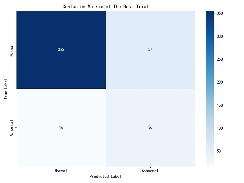
混淆矩阵分析
以下是在高置信度样本子集上的最佳模型的具体表现:
预测为正常 预测为异常
实际为正常 355
57
实际为异常 16
36
依据该矩阵可知,成功检测的有36例;发生漏诊有16例,这是最关键的指标,模型未能识别出16例异常样本。根据代价函数,这部分产生了16 × 15 = 240 16\times15=240 16 × 15 = 240 57 × 1 = 57 57\times1=57 57 × 1 = 57
为了更深入地理解模型的性能,本文对分类报告的各项指标进行解读:
精确率 召回率 F1分数 样本数
正常
0.96
0.86
0.91
412
异常
0.39
0.69
0.50
52
总体准确率 0.84 464
针对“异常”样本:
精确率= 0.39 :在所有被模型预测为“异常”的样本中,只有 39% 是真正的异常。这意味着有较多的假阳性,这也是为了降低更昂贵的假阴性所付出的代价。
召回率 = 0.69 :这是本案例的核心指标之一。它表示在所有真实为“异常”的样本中,模型成功“召回”或识别出了其中的 69%。根据代价函数的设计,模型牺牲了一部分精确率,以换取尽可能高的召回率,从而最大程度地避免漏诊。
针对“正常”样本:
精确率 = 0.96 :在所有被模型预测为“正常”的样本中,有 96% 是真正的正常。这是一个非常高的数值,说明模型给出的“正常”判断具有很高的可靠性。
召回率= 0.86 :在所有真实为“正常”的样本中,有 86% 被模型正确识别。另外的 14% 被错误地划分为“异常”(即假阳性)。
综上所述,模型的AUC值为0.8216 ,表明其在区分异常和正常样本方面具有良好的整体能力。混淆矩阵显示,模型在464个高置信度样本中成功识别了36个异常样本,同时将355个正常样本正确分类为正常。尽管存在57个假阳性,但这是为了最大限度地减少16个假阴性所做的权衡。本文成功构建并优化了一个专门针对女胎NIPT数据异常判定的高级集成模型。该模型通过在筛选后的高置信度数据集上,端到端地学习一个15:1的非对称临床代价函数,实现了在“漏诊”和“误诊”之间的高度定制化的平衡,最终达到了297.0的最低临床代价分数。模型的召回率(69%)显著高于精确率(39%),这与设定的“不惜一切代价避免漏诊”的优化目标一致。
模型各特征的特征重要性
模型的评价
模型的优点
使用生存模型自然地处理删失数据,能提供更符合临床需求的预测结果。
通过融合SVM和XGBoost两种强大的机器学习算法,并进行端到端的自动化超参数调优,模型能够捕捉复杂的非线性关系和特征交互,获得了很高的整体判别能力(AUC=0.8216)。
分箱不是基于先验知识(如传统的“偏瘦/正常/超重”),而是完全由数据驱动,以最大化风险区分度为目标。从结果看,监督式分箱后的KM曲线分离度远优于传统分箱,证明了其有效性。
模型的缺点
多元线性回归模型无法捕捉变量之间复杂的交互作用或非线性模式,因此其预测精度通常不如更复杂的机器学习模型。
最小二乘法容易受到极端异常值的影响,导致模型参数估计产生偏差。
附录
文件列表
文件名
说明
p1\_literature\_based\_analysis.py文献驱动的基础数据分析(问题一)
p1\_relationship\_analysis.py特征相关性分析(问题一)
p1\_xgboost\_analysis.pyXGBoost建模与预测(问题一)
p2\_bmi\_supervised\_binning.pyBMI变量监督分箱处理(问题二)
p2\_eda.py探索性数据分析(问题二)
p2\_noise\_grouped\_sensitivity\_analysis.py分组噪声敏感性分析(问题二)
p2\_plot\_sensitivity\_trends.py敏感性趋势可视化(问题二)
p2\_fuzzy\_interval\_modeling.py模糊区间建模(问题二)
p3\_aft.R加速失效时间(AFT)模型建模(问题三)
p3\_bmi\_group\_plots.pyBMI分组可视化绘图(问题三)
p3\_bmi\_supervised\_binning.pyBMI监督分箱处理(问题三)
p3\_fuzzy\_interval\_modeling.py模糊区间建模(问题三)
p3\_noise\_grouped\_sensitivity\_analysis.py分组噪声敏感性分析(问题三)
p4\_automl\_ensemble\_tuning.pyAutoML集成建模与调参(问题四)
p4\_shap\_analysis.pySHAP模型可解释性分析(问题四)
代码
p1_literature_based_analysis.py
1
2
3
4
5
6
7
8
9
10
11
12
13
14
15
16
17
18
19
20
21
22
23
24
25
26
27
28
29
30
31
32
33
34
35
36
37
38
39
40
41
42
43
44
45
46
47
48
49
50
51
52
53
54
55
56
57
58
59
60
61
62
63
64
65
66
67
68
69
70
71
72
73
74
75
76
77
78
79
80
81
82
83
84
85
86
87
88
89
90
91
92
93
94
95
96
97
98
99
100
101
102
103
104
105
106
107
108
109
110
111
112
113
114
115
116
117
118
119
120
121
122
123
124
125
126
127
128
129
130
131
132
133
134
135
136
137
138
139
140
141
142
143
144
145
146
147
148
149
150
151
152
153
154
155
156
157
158
''' 本脚本根据指定文献的方法,分析Y染色体浓度与孕妇关键特征(年龄、BMI、孕周)之间的关系。 分析流程包括: 1. 孕妇年龄与BMI的相关性分析。 2. Y染色体浓度与孕周的相关性分析。 3. 在不同孕周分组下,校正BMI后,分析Y染色体浓度与孕妇年龄的相关性。 4. 在不同孕周分组下,校正年龄后,分析Y染色体浓度与孕妇BMI的相关性。 新增功能:在进行相关性分析前,会进行正态性检验(Shapiro-Wilk test),并根据检验结果自动选择Pearson或Spearman相关性分析。 ''' import pandas as pdimport numpy as npfrom scipy.stats import pearsonr, shapiro, spearmanrimport redef get_correlation (series1, series2 ):""" 检验两组数据的正态性,并根据结果选择合适的相关性分析方法。 如果两组数据都服从正态分布,则使用Pearson相关系数。 否则,使用Spearman等级相关系数。 """ if len (series1) < 3 or len (series2) < 3 :return np.nan, np.nan, "数据不足 (样本量<3)" 0.05 if shapiro_p1 > alpha and shapiro_p2 > alpha:"Pearson" else :"Spearman" return corr, p_value, methodtry :'../男胎检测数据_filtered.csv' , encoding='gbk' )except UnicodeDecodeError:'../男胎检测数据_filtered.csv' , encoding='utf-8' )'孕周' ] = pd.to_numeric(df['检测孕天数' ], errors='coerce' ) // 7 'Y染色体浓度' , '孕周' , '孕妇BMI' , '年龄' ]for col in ['Y染色体浓度' , '孕妇BMI' , '年龄' ]:print ("--- 数据加载和预处理完成 ---" )print (f"处理后总样本数: {len (analysis_df)} " )print ("转换后的孕周(周数)描述性统计:" )print (analysis_df[['孕周' ]].describe()) print ("-" * 50 + "\n" )print ("--- 2. 孕妇年龄与BMI相关性分析 ---" )'年龄' )['孕妇BMI' ].agg(['median' , 'count' ])'count' ] >= 5 ]'median' ]print (f"孕妇年龄与BMI中值的相关性分析 (样本数>=5的组):" )print (f" - 使用方法: {method} " )print (f" - 相关系数: {corr:.4 f} " )print (f" - p-value: {p_value:.4 f} " )print ("-" * 50 + "\n" )print ("--- 3. Y染色体浓度与孕周相关性分析 ---" )'孕周' )['Y染色体浓度' ].agg(['median' , 'count' ])'count' ] >= 5 ]'median' ]print (f"孕周与Y染色体浓度中值的相关性分析 (样本数>=5的组):" )print (f" - 使用方法: {method} " )print (f" - 相关系数: {corr:.4 f} " )print (f" - p-value: {p_value:.4 f} " )print ("-" * 50 + "\n" )print ("--- 4. Y染色体浓度与孕妇年龄相关性 (校正BMI) ---" )'cfEB' ] = (analysis_df['Y染色体浓度' ] / analysis_df['孕妇BMI' ]) * 1000 11 , 14 , 16 , 18 , 20 , 26 ]'12-14周' , '15-16周' , '17-18周' , '19-20周' , '21-26周' ]'孕周分组' ] = pd.cut(analysis_df['孕周' ], bins=bins, right=True , labels=labels)print ("按孕周分组,分析孕妇年龄与cfEB的相关性:" )for group_name, group_df in analysis_df.groupby('孕周分组' ):'年龄' )['cfEB' ].agg(['median' , 'count' ])'count' ] >= 5 ]print (f"\n孕周组: {group_name} " )if len (age_cfeb_filtered) < 2 :print (" - 数据不足,无法进行相关性分析。" )continue 'median' ]print (f" - 使用方法: {method} " )if pd.isna(corr):continue print (f" - 相关系数: {corr:.4 f} " )print (f" - p-value: {p_value:.4 f} " )print ("-" * 50 + "\n" )print ("--- 5. Y染色体浓度与孕妇BMI相关性 (校正年龄) ---" )'cfEA' ] = (analysis_df['Y染色体浓度' ] / analysis_df['年龄' ]) * 1000 print ("按孕周分组,分析孕妇BMI与cfEA的相关性:" )for group_name, group_df in analysis_df.groupby('孕周分组' ):'孕妇BMI' )['cfEA' ].agg(['median' , 'count' ])'count' ] >= 5 ]print (f"\n孕周组: {group_name} " )if len (bmi_cfea_filtered) < 2 :print (" - 数据不足,无法进行相关性分析。" )continue 'median' ]print (f" - 使用方法: {method} " )if pd.isna(corr):continue print (f" - 相关系数: {corr:.4 f} " )print (f" - p-value: {p_value:.4 f} " )print ("-" * 50 + "\n" )
p1_relationship_analysis.py
1
2
3
4
5
6
7
8
9
10
11
12
13
14
15
16
17
18
19
20
21
22
23
24
25
26
27
28
29
30
31
32
33
34
35
36
37
38
39
40
41
42
43
44
45
46
47
48
49
50
51
52
53
54
55
56
57
58
59
60
61
62
63
64
65
66
67
68
69
70
71
72
73
74
75
76
77
78
79
80
81
82
83
84
85
86
87
88
89
90
91
92
93
94
95
96
97
98
99
100
101
102
103
104
105
106
107
108
109
110
111
112
113
114
115
116
117
118
119
120
121
122
123
124
125
126
127
128
129
130
131
132
133
134
135
136
137
138
139
140
141
142
143
import pandas as pdimport statsmodels.api as smimport reimport pingouin as pgfrom scipy.stats import shapiroimport numpy as nptry :'../男胎检测数据_filtered.csv' , encoding='gbk' )except UnicodeDecodeError:'../男胎检测数据_filtered.csv' , encoding='utf-8' )def clean_gestational_week (gw_str ):if isinstance (gw_str, str ):match = re.search(r'\d+' , gw_str)if match :return int (match .group(0 ))try :return int (gw_str)except (ValueError, TypeError):return None '检测孕周_cleaned' ] = df['检测孕天数' ].apply(clean_gestational_week)'Y染色体浓度' , '检测孕周_cleaned' , '孕妇BMI' , '年龄' ]'Y染色体浓度' ] = pd.to_numeric(analysis_df['Y染色体浓度' ])'检测孕周_cleaned' ] = pd.to_numeric(analysis_df['检测孕周_cleaned' ])'孕妇BMI' ] = pd.to_numeric(analysis_df['孕妇BMI' ])'年龄' ] = pd.to_numeric(analysis_df['年龄' ])print ("--- 正在进行特征工程 ---" )0.05 print ("--- 正态性检验 (Shapiro-Wilk) ---" )print ("原假设 (H0): 数据服从正态分布" )print (f"显著性水平 (alpha) = {alpha} \n" )True for column in ['Y染色体浓度' , '检测孕周_cleaned' , '孕妇BMI' , '年龄' ]:print (f"变量: {column} " )print (f" - 检验统计量: {stat:.4 f} " )print (f" - p-value: {p_value:.4 f} " )if p_value > alpha:print (f" - 结论: p > {alpha} ,不能拒绝原假设,数据可视为服从正态分布。" )else :False print (f" - 结论: p <= {alpha} ,拒绝原假设,数据不服从正态分布。" )print ("-" * 30 )print ("\n--- 偏相关系数分析 ---" )if not all_normal:print ("*** 警告: 由于部分或全部数据未通过正态性检验,将使用Spearman方法进行相关性分析。***" )print ("--- Spearman 偏相关系数 (基于秩次) ---" )'Y染色体浓度' , '检测孕周_cleaned' , '孕妇BMI' , '年龄' ]].rank().pcorr()else :print ("--- Pearson 偏相关系数 ---" )'Y染色体浓度' , '检测孕周_cleaned' , '孕妇BMI' , '年龄' ]].pcorr()print (partial_corr_df)print ("\n" )'Y染色体浓度' ]'检测孕周_cleaned' ,'孕妇BMI' ,'年龄' ]]print ("\n--- 改造后的线性回归模型摘要 ---" )print (model_engineered.summary())print ("\n" )print ("--- 结果解读 ---" )print (f"调整后的R平方 (Adj. R-squared): {r_squared:.4 f} " )print (f"F统计量 p值: {f_pvalue:.4 f} " )print ("\n系数及其p值:" )for var in coefficients.index:print (f" {var} : {coefficients[var]:.4 f} (p-value: {p_values[var]:.4 f} )" )print ("\n" )print (f"显著性水平 (alpha) = {alpha} " )if f_pvalue < alpha:print ("整体模型在统计上是显著的 (F检验 p-value < 0.05)。" )else :print ("整体模型在统计上不显著 (F检验 p-value >= 0.05)。" )print ("\n各系数显著性:" )for var in p_values.index:if var == 'const' : continue if p_values[var] < alpha:print (f"- 特征 '{var} ' 在统计上是显著的。" )else :print (f"- 特征 '{var} ' 在统计上不显著。" )
p1_xgboost_analysis.py
1
2
3
4
5
6
7
8
9
10
11
12
13
14
15
16
17
18
19
20
21
22
23
24
25
26
27
28
29
30
31
32
33
34
35
36
37
38
39
40
41
42
43
44
45
46
47
48
49
50
51
52
53
54
55
56
57
58
59
60
61
62
63
64
65
66
67
68
69
70
71
72
73
74
75
76
77
78
79
80
81
82
83
84
85
86
87
88
89
90
91
92
93
94
95
96
97
98
99
100
101
102
103
104
105
106
107
108
109
import pandas as pdimport xgboost as xgbimport seaborn as snsimport matplotlib.pyplot as pltfrom sklearn.model_selection import cross_val_score, GridSearchCVfrom sklearn.inspection import PartialDependenceDisplayimport redef main ():print ("--- 1. 开始加载和准备数据 ---" )try :'../男胎检测数据_filtered.csv' , encoding='gbk' )except UnicodeDecodeError:'../男胎检测数据_filtered.csv' , encoding='utf-8' )def clean_gestational_week (gw_str ):if isinstance (gw_str, str ):match = re.search(r'\d+' , gw_str)if match : return int (match .group(0 ))try : return int (gw_str)except (ValueError, TypeError): return None '检测孕周_cleaned' ] = df['检测孕天数' ].apply(clean_gestational_week)'Y染色体浓度' , '检测孕周_cleaned' , '孕妇BMI' , '年龄' ]'检测孕周_cleaned' , '孕妇BMI' , '年龄' ]]'Y染色体浓度' ]print ("数据加载和准备完成。" )'font.sans-serif' ] = ['SimHei' ]'axes.unicode_minus' ] = False 'reg:squarederror' ,42 'n_estimators' : [100 , 150 , 200 ],'max_depth' : [3 , 4 , 5 ],'learning_rate' : [0.05 , 0.1 ],'subsample' : [0.8 , 0.9 ],'colsample_bytree' : [0.8 , 0.9 ]print ("\n--- 3. 使用GridSearchCV进行自动调参 ---" )5 ,'r2' ,1 ,1 print (f"\n找到的最佳参数: {grid_search.best_params_} " )print (f"使用最佳参数在交叉检验中的最佳R²分数: {grid_search.best_score_:.4 f} " )print ("\n--- 4. 最佳模型已在全部数据上完成训练 ---" )print ("最终模型已准备好用于分析。" )print ("\n--- 5. 分析特征重要性 ---" )'Feature' : feature_names,'Importance' : importances'Importance' , ascending=False )print ("各特征重要性排序:" )print (importance_df)10 , 6 ))'Importance' , y='Feature' , data=importance_df)'特征重要性排序 (正则化XGBoost)' )print ("\n--- 6. 生成所有特征的部分依赖图 ---" )0 , 1 , 2 ] 3 ,30 ,'所有特征对Y染色体浓度的部分依赖性 (正则化XGBoost)' , size=16 )0.9 )print ("\n分析完成。" )if __name__ == '__main__' :
p2_bmi_supervised_binning.py
1 2 3 4 5 6 7 8 9 10 11 12 13 14 15 16 17 18 19 20 21 22 23 24 25 26 27 28 29 30 31 32 33 34 35 36 37 38 39 40 41 42 43 44 45 46 47 48 49 50 51 52 53 54 55 56 57 58 59 60 61 62 63 64 65 66 67 68 69 70 71 72 73 74 75 76 77 78 79 80 81 82 83 84 85 86 87 88 89 90 91 92 93 94 95 96 97 98 99 100 101 102 103 104 105 106 107 108 109 110 111 112 113 114 115 116 117 118 119 120 121 122 123 124 125 126 127 128 129 130 131 132 133 134 135 136 137 138 139 140 141 142 143 144 145 146 147 148 149 150 151 152 153 154 155 156 157 158 159 160 161 162 163 164 165 166 167 168 169 170 171 172 173 174 175 176 177 178 179 180 181 182 183 184 185 186 187 188 189 190 191 192 193 194 195 196 197 198 199 200 201 202 203 204 205 206 207 208 209 210 211 212 213 214 215 216 217 218 219 220 221 222 223 224 225 226 227 228 229 230 231 232 233 234 235 236 237 238 239 240 241 242 243 244 245 246 247 248 249 250 251 252 253 254 255 256 257 258 259 260 261 262 263 264 265 266 267 268 269 270 271 272 273 274 275 276 277 278 279 280 281 282 283 284 285 286 287 288 289 290 291 292 293 294 295 296 297 298 299 300 301 302 303 304 305 306 307 308 309 310 311 312 313 314 315 316 317 318 319 320 321 322 323 324 325 326 327 328 329 330 331 332 333 334 335 336 337 338 339 340 341 342 343 344 345 346 347 348 349 350 351 352 353 354 355 356 357 358 359 360 361 362 363 364 365 366 367 368 369 370 371 372 373 374 375 376 377 378 379 380 381 382 383 384 385 386 387 388 389 390 391 392 393 394 395 396 397 398 399 400 401 402 403 404 405 406 407 408 409 410 411 412 413 414 415 416 417 418 419 420 421 422 423 424 425 426 427 428 429 430 431 432 433 434 435 436 437 438 439 440 441 442 443 444 445 446 447 448 449 450 451 452 453 454 455 456 457 458 459 460 461 462 463 464 465 466 467 468 469 470 471 472 473 474 475 476 477 478 479 480 481 482 483 484 485 486 487 488 489 490 491 492 493 494 495 496 497 498 499 500 501 502 503 504 505 506 507 508 509 510 511 512 513 514 515 516 517 518 519 520 521 522 523 524 525 526 527 528 529 530 531 532 533 534 535 536 537 538 539 540 541 542 543 544 545 546 547 548 549 550 551 552 553 554 555 556 557 558 559 560 561 562 563 564 565 566 567 568 569 570 571 572 573 574 575 576 577 578 579 580 581 582 583 584 585 586 587 588 589 590 591 592 593 594 595 596 597 598 599 600 601 602 603 604 605 606 607 608 609 610 611 612 613 614 615 616 617 618 619 620 621 622 623 624 625 626 627 628 629 630 631 632 633 634 635 636 637 638 639 640 641 642 643 644 645 646 647 648 649 650 651 652 653 654 655 656 657 658 659 660 661 662 663 664 665 666 667 668 669 670 671 672 673 674 675 676 677 678 679 680 681 682 683 684 685 686 687 688 689 690 691 692 693 694 695 696 697 698 699 700 701 702 703 704 705 706 707 708 709 710 711 712 713 714 715 716 717 718 719 720 721 722 723 724 725 726 727 728 729 730 731 732 733 734 735 736 737 738 739 740 741 742 743 744 745 746 747 748 749 750 751 752 753 754 755 756 757 758 759 760 761 762 763 764 765 766 767 768 769 770 771 772 773 774 775 776 777 778 779 780 781 782 783 784 785 786 787 788 789 790 791 792 793 794 795 796 797 798 799 800 801 802 803 804 805 806 807 808 809 810 811 812 813 814 815 816 817 818 819 820 821 822 823 824 825 826 827 828 829 830 831 832 833 834 835 836 837 838 839 840 841 842 843 844 845 846 847 848 849 850 851 852 853 854 855 856 857 858 859 860 861 862 863 864 865 866 867 868 869 870 871 872 873 874 875 876 877 878 879 880 881 882 883 884 885 886 887 888 889 890 891 892 893 894 895 896 897 898 899 900 901 902 903 904 905 906 907 908 909 910 911 912 913 914 915 916 917 918 919 920 921 922 923 924 925 926 927 928 929 930 931 932 933 934 935 936 937 938 939 940 941 942 943 944 945 946 947 948 949 950 951 952 953 954 955 956 957 958 959 960 961 962 963 964 965 966 967 968 969 970 971 972 973 974 975 976 977 978 979 980 981 982 983 984 985 986 987 988 989 990 991 992 993 994 995 996 997 998 999 1000 1001 1002 1003 1004 1005 1006 1007 1008 1009 1010 1011 1012 1013 1014 1015 1016 1017 1018 1019 1020 """ 生存导向监督分箱(BMI)— 支持“区间删失 + 多重插补(MI)”与自适应插补、log-rank 显著性 - 固定为4组 + 可复现 + 单调化 + 稳健切分 + 切点持久化 - 支持 time-dependent AUC(scikit-survival,不装则跳过) - 新增:对左删失占比高的 BMI 段,自适应采用“向右偏重的插补(trunc_exp)并把左界抬到 10 周” - 新增:相邻 BMI 组的 log-rank 检验(基于 MI 多次插补,Fisher 法合并 p 值),导出 CSV 运行: python p2_bmi_supervised_binning.py 输出目录: ./outputs_binning """ import osimport jsonimport randomimport warningsimport numpy as npimport pandas as pdimport matplotlib.pyplot as plt'font.sans-serif' ] = ['SimHei' ]'axes.unicode_minus' ] = False from lifelines import CoxPHFitter, KaplanMeierFitterfrom lifelines.utils import k_fold_cross_validationfrom lifelines.statistics import logrank_testfrom patsy import dmatrixfrom sklearn.tree import DecisionTreeRegressorfrom sklearn.isotonic import IsotonicRegressiontry :from sksurv.metrics import cumulative_dynamic_aucfrom sksurv.util import Surv as SKSurvTrue except Exception:False "未安装 scikit-survival,将跳过 time-dependent AUC。pip install scikit-survival" )try :from scipy.stats import chi2True except Exception:False "未安装 SciPy,将无法用 Fisher 法合并 p 值。pip install scipy" )42 def set_global_seed (seed: int = 42 ):"PYTHONHASHSEED" ] = str (seed)"./eda_outputs/patient_level_summary.csv" "../男胎检测数据_filtered.csv" "./outputs_binning" 10.0 , 30.0 801 0.90 , 0.95 ]0.95 True 4 40 2.0 20 True 5 10 4 3 None 0.0 , 0.02 , 0.05 , 0.1 , 0.2 ] 5 True 20 "uniform" True 6.0 True 0.6 "trunc_exp" 10.0 20 10.0 , 14.0 )"孕妇代码" "检测孕天数" "检测日期" "Y染色体浓度" "孕妇BMI" "身高" "体重" 0.04 def to_num (s ): return pd.to_numeric(s, errors="coerce" )def derive_week (s_days ): return to_num(s_days) / 7.0 def compute_bmi (h_cm, w_kg ):100.0 return w / (h_m ** 2 )def parse_y_as_fraction (s ):if s.dtype == object :str ).str .strip()if s_str.str .contains("%" ).any ():str .replace("%" ,"" ).str .replace("," ,"" ), errors="coerce" )return vals / 100.0 "coerce" )if finite.size >= 10 :95 )if 1.0 < q95 <= 100.0 :return y / 100.0 return ydef safe_min (a ):return float (np.nanmin(a)) if np.isfinite(a).any () else np.nandef safe_max (a ):return float (np.nanmax(a)) if np.isfinite(a).any () else np.nandef build_patient_interval_from_raw (raw_csv, detection_lower_bound=DETECTION_LOWER_BOUND ):if COL_GA_DAYS not in df.columns or COL_PATIENT not in df.columns or COL_Y_CONC not in df.columns:raise ValueError("原始CSV缺少必要列(孕妇代码/检测孕天数/Y染色体浓度)。" )"孕周" ] = derive_week(df[COL_GA_DAYS])if COL_DATE in df.columns:"coerce" )"Y_frac" ] = parse_y_as_fraction(df[COL_Y_CONC])"有效测量" ] = ~df["Y_frac" ].isna()"达标" ] = df["有效测量" ] & (df["Y_frac" ] >= THRESH_Y_FRAC)if COL_BMI in df.columns:"BMI_num" ] = to_num(df[COL_BMI])else :"BMI_num" ] = np.nanif df["BMI_num" ].isna().any () and (COL_HEIGHT in df.columns) and (COL_WEIGHT in df.columns):"BMI_num" ].isna(), "BMI_num" ] = calc[df["BMI_num" ].isna()]"孕周" ] + ([COL_DATE] if COL_DATE in df.columns else [])for pid, g in df.groupby(COL_PATIENT, dropna=False ):"BMI_num" ].dropna().iloc[0 ] if g["BMI_num" ].notna().any () else np.nan"有效测量" ]].copy()"孕周" ].values"达标" ].values.astype(bool )if len (times) == 0 :"missing" else :0 ]if len (pos_idx) > 0 :int (pos_idx[0 ])0 ]if len (neg_before) > 0 :float (times[neg_before[-1 ]])float (times[first_pos_i])if R < L:"interval" else :float (detection_lower_bound)float (times[first_pos_i])if R < L:max (R - 1e-3 , detection_lower_bound)"left" else :float (times[-1 ])"right" "patient_id" : pid, "BMI" : bmi, "L" : L, "R" : R, "ctype" : ctypereturn df_intdef _rand_trunc_expon (L, R, scale=2.0 ):if not np.isfinite(R):1.0 - np.exp(-(R - L) / scale)if denom <= 1e-12 :return float ((L + R) / 2.0 )1 - U * denom) + Lreturn float (min (max (t, L + 1e-6 ), R))def sample_time_from_interval (L, R, left_lower_bound=DETECTION_LOWER_BOUND, method="uniform" ):if not np.isfinite(R):return np.nanif not np.isfinite(L):float (left_lower_bound)float (L); R_eff = float (R)if R_eff <= L_eff:return float (R_eff)if method == "uniform" :return float (np.random.uniform(L_eff, R_eff))else :return _rand_trunc_expon(L_eff, R_eff, scale=2.0 )def multiple_imputations_from_intervals (df_int, M=MI_M, method=MI_SAMPLING, left_lower_bound=DETECTION_LOWER_BOUND ):"ctype" ].isin(["interval" , "left" , "right" ])for m in range (M):for _, r in base.iterrows():"ctype" ]; BMI = r["BMI" ]; pid = r["patient_id" ]; L, R = r["L" ], r["R" ]if ctype in ["interval" , "left" ] and np.isfinite(R):"patient_id" : pid, "BMI" : BMI, "time" : t, "event" : 1 })elif ctype == "right" and np.isfinite(L):"patient_id" : pid, "BMI" : BMI, "time" : float (L), "event" : 0 })else :continue "time" ] >= 6 ) & (df_m["time" ] <= 40 )]"event" ] = df_m["event" ].astype(int )True ))return dfsdef bins_from_cuts (x, cuts ):if len (cuts) == 0 :else :for i in range (len (bins)-1 ):1 ]f"[{round (a,1 ) if np.isfinite(a) else '-inf' } , {round (b,1 ) if np.isfinite(b) else '+inf' } )" )1 :-1 ], right=False )return pd.Series([labels[i] for i in idx], index=x.index), bins, labelsdef parse_label_left (label: str ) -> float :"," )[0 ][1 :].strip()return float (left.replace("-inf" , "-1e9" ))def compute_left_censor_rates (df_int, labels_series ):for g, idxs in labels_series.groupby(labels_series).groups.items():len (sub)if n == 0 :else :float ((sub["ctype" ] == "left" ).sum ()) / n"group" : g, "n" : n, "left_censor_rate" : rate})"group" , key=lambda s: s.map (parse_label_left)).reset_index(drop=True )return resdef multiple_imputations_adaptive (df_int, labels_series, left_rate_df, threshold=LEFT_CENSOR_RATE_THRESHOLD, M=ADAPTIVE_M, method_default=MI_SAMPLING, method_high=ADAPTIVE_METHOD_HIGH, lb_default=DETECTION_LOWER_BOUND, lb_high=ADAPTIVE_LB_HIGH ):dict (zip (left_rate_df["group" ], left_rate_df["left_censor_rate" ]))for m in range (M):for idx, r in df_int.iterrows():if r["ctype" ] not in ["interval" , "left" , "right" ]:continue if idx in labels_series.index else None 0.0 )is not None ) and (np.isfinite(rate)) and (rate >= threshold)if use_high else method_defaultif use_high else lb_default"patient_id" ]; BMI = r["BMI" ]; L, R, ct = r["L" ], r["R" ], r["ctype" ]if ct in ["interval" , "left" ] and np.isfinite(R):"patient_id" : pid, "BMI" : BMI, "time" : t, "event" : 1 })elif ct == "right" and np.isfinite(L):"patient_id" : pid, "BMI" : BMI, "time" : float (L), "event" : 0 })else :continue "time" ] >= 6 ) & (df_m["time" ] <= 40 )]"event" ] = df_m["event" ].astype(int )True ))return dfsdef km_quantile_time (durations, events, target_S ):"KM_estimate" :"S" ,"timeline" :"t" })"t" )"S" ] <= target_S]return float (hit["t" ].iloc[0 ]) if len (hit) else np.nandef per_group_km_quantiles (df, group_col, p_list ):for g, sub in df.dropna(subset=["time" ,"BMI" ]).groupby(group_col):"group" : str (g), "n" : len (sub)}if len (sub) >= 20 :for p in p_list:f"KM_t{int (p*100 )} " ] = km_quantile_time(sub["time" ].values, sub["event" ].values, target_S=1.0 - p)else :for p in p_list:f"KM_t{int (p*100 )} " ] = np.nanreturn pd.DataFrame(rows)def group_km_recommendations_from_imputations (imputed_sets, cuts_final, p=MAIN_P ):for df_m in imputed_sets:"BMI" ], cuts_final)"group" , [p])f"KM_t{int (p*100 )} " for _, r in rec.iterrows():"group" ], []).append(r[col])for g, L in label_vals.items():for v in L if np.isfinite(v)])"group" : g, f"KM_t{int (p*100 )} _MI_med" : (float (np.median(arr)) if len (arr) > 0 else np.nan)})"group" , key=lambda s: s.map (parse_label_left)).reset_index(drop=True )return outdef predict_tp_from_cox (cph, df_feat, p=0.90 , time_grid=None ):if time_grid is None :1.0 - pfor col in surv.columns:0 ]if len (hit) == 0 else time_grid[hit[0 ]])return pd.Series(t_list, index=df_feat.index)def make_bmi_spline (bmi_series, bmi_center, df=SPLINE_DF, degree=SPLINE_DEGREE ):f"bs(BMI_centered, df={df} , degree={degree} , include_intercept=False)" ,"BMI_centered" : (bmi_series - bmi_center).values},'dataframe' return Xsdef extract_tree_cuts_1d (tree: DecisionTreeRegressor ):sorted ([float (t) for t in thr if t != -2.0 ])return cutsdef apply_min_width (cuts, min_width=2.0 ):if not cuts:return []0 ]]for c in cuts[1 :]:if c - kept[-1 ] >= min_width:return keptdef merge_small_bins (df_labels, label_col, min_samples=40 ):sorted (df_labels[label_col].unique(), key=parse_label_left)def neighbors (idx ):1 ] if idx-1 >= 0 else None 1 ] if idx+1 < len (labels_order) else None return left, rightTrue while changed:False for lab in labels_order if counts.get(lab, 0 ) < min_samples]for lab in smalls:if lab not in labels_order:continue if L is None and R is None :continue 1 )1 )if (cL >= cR and L is not None ) else (R if R is not None else L)0 ) + counts.get(lab, 0 )0 True break return df_labels[label_col]def canonicalize_from_labels (x_series, labels_series ):sorted (set (parse_label_left(l) for l in uniq_labels))for v in lefts if v > -1e8 ]return cuts_final, labels_final, bins_edges, labels_textdef evaluate_bins_mae (bmi, y_true, labels ):"BMI" : bmi, "y" : y_true, "label" : labels})"label" )["y" ].median().to_dict()"label" ].map (preds).astype(float )abs (df_tmp["y" ].values - y_hat.values))"label" ].value_counts().to_dict()return mae, sizesdef fit_cox_with_cv_penalizer (cox_df, penalizer_grid, duration_col="time" , event_col="event" , k=5 ):None for pen in penalizer_grid:float (pen))try :False )"concordance_index" float (np.mean(scores))except Exception:float (pen), mean_c))if np.isfinite(mean_c) and mean_c > best_c:float (pen)if best_pen is None :0.0 return best_pen, resultsdef time_dependent_auc_curve (df, lower=10.0 , upper=30.0 , n_points=40 , kfold=5 , penalizer=0.05 ):if not HAS_SK_SURV:return None , None , None "BMI" ,"time" ,"event" ]).copy()"time" ] >= 6 ) & (df["time" ] <= 40 )]if len (df) < 50 :"样本过少,跳过 AUC 评估。" )return None , None , None "BMI" ].mean()"bs(BMI_centered, df=4, degree=3, include_intercept=False)" ,"BMI_centered" : (df["BMI" ] - BMI_CENTER).values}, return_type='dataframe' )"time" ,"event" ]].copy()len (df)); np.random.shuffle(idx)0 for i in range (kfold):if len (train_idx) < 20 or len (test_idx) < 20 : continue True ),True )], axis=1 )try :"time" , event_col="event" , show_progress=False )except Exception as e:f"Cox 拟合失败 fold {i+1 } : {e} " ); continue "event" ].astype(bool ).values,"time" ].values)"event" ].astype(bool ).values,"time" ].values)float (np.min (y.iloc[test_idx]["time" ].values))float (np.max (y.iloc[test_idx]["time" ].values))1e-8 ) & (times_global < tmax - 1e-8 )if not np.any (mask): continue try :except ValueError:1e-3 if not np.any (mask2): continue float )1 if used_fold == 0 :"无可用折进行 AUC 评估。" ); return None , None , None 0 )0 )7.5 ,4.5 ))2 , label="Mean AUC(t)" )0.5 ), np.nan_to_num(hi, nan=1.0 ), alpha=0.2 , label="±1 SD" )0.5 , 1.0 ); plt.xlabel("孕周(周)" ); plt.ylabel("AUC(t)" )"Time-dependent AUC(Cox + BMI 样条,K折,自动裁剪时域)" )0.3 ); plt.legend()"auc_curve.png" ), dpi=180 ); plt.close()"t" : times_global, "auc_mean" : mean_auc, "auc_sd" : std_auc})"auc_curve.csv" ), index=False , encoding="utf-8-sig" )return times_global, mean_auc, std_aucdef main ():True )"bmi_supervised_bins_cuts.json" )if os.path.exists(meta_path_prev):try :with open (meta_path_prev, "r" , encoding="utf-8" ) as f:print (f"[INFO] 上一次运行 seed={prev.get('seed' )} , cuts_final={prev.get('chosen' ,{} ).get('cuts_final')}" )except Exception as e:print ("[WARN] 读取上一次 JSON 失败:" , e)None "exact" None if USE_INTERVAL_MI and os.path.exists(RAW_CSV):print ("[INFO] 使用区间删失 + 多重插补(MI)路径..." )"interval_mi" "patient_level_intervals.csv" )False , encoding="utf-8-sig" )print (f"[INFO] 已保存区间数据: {out_int_csv} (n={len (df_int)} )" )print (f"[INFO] 生成多重插补数据集 M={len (imputed_sets)} " )None None None for m_idx, df_m in enumerate (imputed_sets):if len (df_m) == 0 : continue "BMI" ].mean()"BMI" ], BMI_CENTER, df=SPLINE_DF, degree=SPLINE_DEGREE)"time" ,"event" ]].reset_index(drop=True ),True )], axis=1 )if COX_PENALIZER is None :if (m_idx == 0 ) or (not CV_ONCE_FOR_MI):"time" , event_col="event" , k=CV_FOLDSfloat (best_pen)print (f"[MI {m_idx+1 } ] Cox penalizer CV: {pen_cv} -> best={best_pen} " )else :else :float (COX_PENALIZER)if m_idx == 0 :print (f"[MI {m_idx+1 } ] Cox penalizer fixed to: {best_pen} " )"time" , event_col="event" , show_progress=False )for p in P_LIST:f"pred_t{int (p*100 )} " ] = predict_tp_from_cox(cph, X_spline, p=p, time_grid=time_grid)True ), pd.DataFrame(pred_cols).reset_index(drop=True )], axis=1 )"BMI" ] = df_m["BMI" ].valuesif agg_preds is None :"patient_id" ,"BMI" ] + [f"pred_t{int (p*100 )} " for p in P_LIST]].copy()for p in P_LIST:f"pred_t{int (p*100 )} _list" ] = agg_preds[f"pred_t{int (p*100 )} " ].apply(lambda x: [x])else :"patient_id" )"patient_id" )for p in P_LIST:f"pred_t{int (p*100 )} " ]f"pred_t{int (p*100 )} _list" ]f"pred_t{int (p*100 )} _list" ] = [if (i < len (vals)) else lst.iloc[i]for i in range (len (lst))if m_idx == 0 :try :"time" , event_col="event" ,"concordance_index" )print (f"[MI {m_idx+1 } ] {CV_FOLDS} -fold C-index: mean={np.mean(scores):.3 f} , std={np.std(scores):.3 f} " )except Exception as e:print ("[MI] 交叉验证跳过:" , e)if agg_preds is None :raise RuntimeError("多重插补生成的预测为空,请检查数据。" )for p in P_LIST:f"pred_t{int (p*100 )} _list" ]f"pred_t{int (p*100 )} " ] = lists.apply(lambda L: np.nanmedian([v for v in L if np.isfinite(v)]) if isinstance (L, list ) and len (L)>0 else np.nan"patient_id" : agg_preds["patient_id" ],"BMI" : agg_preds["BMI" ]for p in P_LIST:f"pred_t{int (p*100 )} " ] = agg_preds[f"pred_t{int (p*100 )} " ].values"time" ] = df_pred_first["time" ].values"event" ] = df_pred_first["event" ].valueselse :print ("[INFO] 使用原始(把首次达标视为精确事件)的路径..." )"exact" if os.path.exists(PATIENT_CSV):if "patient_id" not in df_pat.columns:if "孕妇代码" in df_pat.columns:"孕妇代码" :"patient_id" })else :"patient_id" ] = np.arange(len (df_pat))if "BMI" not in df_pat.columns and "BMI_num" in df_pat.columns:"BMI_num" :"BMI" })else :for _, r in df_int_tmp.iterrows():if r["ctype" ] in ["interval" , "left" ] and np.isfinite(r["R" ]):"patient_id" : r["patient_id" ], "BMI" : r["BMI" ], "time" : r["R" ], "event" : 1 })elif r["ctype" ] == "right" and np.isfinite(r["L" ]):"patient_id" : r["patient_id" ], "BMI" : r["BMI" ], "time" : r["L" ], "event" : 0 })"patient_id" ,"BMI" ,"time" ,"event" ]for k in needed:if k not in df_pat.columns:raise ValueError(f"数据缺列:{k} " )"BMI" ,"time" ,"event" ])"time" ] >= 6 ) & (df["time" ] <= 40 )]"event" ] = df["event" ].astype(int )"BMI" ].mean()"BMI" ], BMI_CENTER, df=SPLINE_DF, degree=SPLINE_DEGREE)"time" ,"event" ]].reset_index(drop=True ),True )], axis=1 )if COX_PENALIZER is None :"time" , event_col="event" , k=CV_FOLDSfloat (best_pen)print (f"Cox penalizer CV: {pen_cv} -> best={best_pen} " )else :float (COX_PENALIZER)print (f"Cox penalizer fixed to: {penalizer} " )"time" , event_col="event" , show_progress=False )try :"time" , event_col="event" ,"concordance_index" )print (f"{CV_FOLDS} -fold C-index: mean={np.mean(scores):.3 f} , std={np.std(scores):.3 f} " )except Exception:pass for p in P_LIST:f"pred_t{int (p*100 )} " ] = predict_tp_from_cox(cph, X_spline_train, p=p, time_grid=time_grid)True ), pd.DataFrame(pred).reset_index(drop=True )], axis=1 )f"pred_t{int (MAIN_P*100 )} " "BMI" ].valuesTrue , out_of_bounds="clip" )"t_main_mono" ] = y95_fitif MONOTONE_Q90 and "pred_t90" in df_pred.columns:"pred_t90" ].fillna(TIME_UPPER).values"t90_mono" ] = y90_fitelse :"t90_mono" ] = df_pred.get("pred_t90" , pd.Series(np.nan, index=df_pred.index))"t_main_mono" ].values"BMI" ]].valuesfor alpha in ccp_alphas:float (alpha),"BMI" ], cuts)"label" : labels_series})"label" , MIN_SAMPLES_PER_BIN)"BMI" ], labels_merged)"BMI" ].values, y_target, labels_final.values)len (set (labels_final.values))"alpha" : float (alpha),"cuts_raw" : cuts_raw,"cuts_after_minwidth" : cuts,"cuts_final" : cuts_final,"bins_edges_final" : [None if not np.isfinite(b) else float (b) for b in bins_edges_final],"n_bins_final" : n_bins_final,"mae" : float (mae),"sizes" : {k:int (v) for k,v in sizes.items()},"labels_series_final" : labels_final.copy()def dist_to_required (n ): return abs (n - REQUIRED_BINS)for c in candidates if c["n_bins_final" ] == REQUIRED_BINS]if exact:sorted (exact, key=lambda c: (c["mae" ]))[0 ]else :sorted (candidates, key=lambda c: (dist_to_required(c["n_bins_final" ]), c["mae" ]))[0 ]"BMI_bin_supervised" ] = chosen["labels_series_final" ].valuesdef enforce_bins_and_min_samples ():"label" : df_pred["BMI_bin_supervised" ]})"label" , max (MIN_SAMPLES_PER_BIN, PLOT_MIN_SAMPLES))"BMI" ], labels_merged2)len (set (labels_final2.values))return labels_final2, cuts_final2, bins_edges_final2, n_bins2if n_bins2 != REQUIRED_BINS:None for cnd in sorted (candidates, key=lambda c: (dist_to_required(c["n_bins_final" ]), c["mae" ])): "BMI_bin_supervised" ] = cnd["labels_series_final" ].valuesif n_bins2 == REQUIRED_BINS:break if alt is not None :"BMI_bin_supervised" ] = labels_final2.values"cuts_final" ] = cuts_final2"bins_edges_final" ] = [None if not np.isfinite(b) else float (b) for b in bins_edges_final2]len (set (df_pred["BMI_bin_supervised" ]))print (f"[INFO] 最终组数: {n_bins_final} (目标 {REQUIRED_BINS} )" )"BMI_bin_supervised" , P_LIST)"BMI_bin_supervised" )[["pred_t90" ,"pred_t95" ,"t_main_mono" ,"t90_mono" ]].median().reset_index() \"pred_t90" :"Cox_pred_t90_median" ,"pred_t95" :"Cox_pred_t95_median" ,"t_main_mono" :"Cox_t_main_mono_median" ,"t90_mono" :"Cox_t90_mono_median" })"group" , right_on="BMI_bin_supervised" , how="left" ).drop(columns=["BMI_bin_supervised" ])"group" , key=lambda s: s.map (parse_label_left)).reset_index(drop=True )"Cox_t_main_mono_median" ].apply(lambda x: np.nan if pd.isna(x) else round (x*2 )/2 ).valuesfor i in range (1 , len (rec)):if not np.isnan(rec[i-1 ]) and (np.isnan(rec[i]) or rec[i] < rec[i-1 ]):1 ]"recommended_week" ] = recif ADAPTIVE_ENABLE and (df_int is not None ):"BMI" ], chosen["cuts_final" ])"left_censor_rates_by_group.csv" ), index=False , encoding="utf-8-sig" )print ("\n[INFO] 左删失比例(按最终 BMI 组):" )print (left_rates.to_string(index=False ))"cuts_final" ], p=MAIN_P)f"KM_t{int (MAIN_P*100 )} _MI_med" ].values.copy()for i in range (1 , len (rec_vals)):if np.isfinite(rec_vals[i-1 ]) and (np.isnan(rec_vals[i]) or rec_vals[i] < rec_vals[i-1 ]):1 ]if np.isnan(v) else round (v*2 )/2 for v in rec_vals])"recommended_week_adaptive" ] = rec_vals"recommendations_adaptive.csv" ), index=False , encoding="utf-8-sig" )print ("\n[INFO] 自适应插补后的组内 KM Q95(插补中位数)与推荐:" )print (rec_adapt.to_string(index=False ))"left_rates" ] = left_rates"rec_adapt" ] = rec_adaptsorted (rec_adapt["group" ].tolist(), key=parse_label_left)1 ]) for i in range (len (ordered_groups)-1 )]for gL, gR in pairs:for df_m in imps_adapt:"BMI" ], chosen["cuts_final" ])if len (subL) < 5 or len (subR) < 5 :continue try :"time" ], subR["time" ],"event" ], event_observed_B=subR["event" ])float (res.p_value))except Exception:continue if len (p_list) == 0 :else :float (np.median(p_list))if HAS_SCIPY:2.0 * np.sum (np.log(np.clip(p_list, 1e-300 , 1.0 )))2 * len (p_list)float (1.0 - chi2.cdf(stat, df_chi))else :"group_left" : gL, "group_right" : gR,"n_imputations" : len (p_list),"p_median" : p_median, "p_fisher" : p_fisher})"logrank_adjacent_adaptive.csv" ), index=False , encoding="utf-8-sig" )print ("\n[INFO] 相邻 BMI 组 log-rank(自适应 MI,Fisher 合并 p):" )print (df_lr.to_string(index=False ))"bmi_supervised_bins_summary.csv" )False , encoding="utf-8-sig" )print (f"\n已保存分箱汇总:{out_csv} " )print (summary.to_string(index=False ))float (df_pred["BMI" ].min ()); bmi_max = float (df_pred["BMI" ].max ())"seed" : SEED, "mode" : mode_used,"time_grid" : {"lower" : TIME_LOWER, "upper" : TIME_UPPER, "n_points" : N_TIME_POINTS},"main_quantile" : MAIN_P, "monotone_q90" : MONOTONE_Q90,"required_bins" : REQUIRED_BINS, "min_samples_per_bin" : MIN_SAMPLES_PER_BIN, "min_bin_width" : MIN_BIN_WIDTH,"tree_base" : {"max_depth" : TREE_BASE_MAX_DEPTH, "min_samples_leaf" : TREE_BASE_MIN_SAMPLES_LEAF, "random_state" : TREE_RANDOM_STATE},"interval_mi" : {"use_interval_mi" : USE_INTERVAL_MI, "mi_M" : MI_M, "mi_sampling" : MI_SAMPLING,"cv_once_for_mi" : CV_ONCE_FOR_MI, "detection_lower_bound" : DETECTION_LOWER_BOUND,"adaptive" : {"enabled" : ADAPTIVE_ENABLE,"left_censor_rate_threshold" : LEFT_CENSOR_RATE_THRESHOLD,"method_high" : ADAPTIVE_METHOD_HIGH,"lb_high" : ADAPTIVE_LB_HIGH,"adaptive_M" : ADAPTIVE_M"cox" : {"spline_df" : SPLINE_DF, "spline_degree" : SPLINE_DEGREE},"data" : {"bmi_min" : bmi_min, "bmi_max" : bmi_max, "n" : int (len (df_pred))},"chosen" : {"cuts_final" : [round (x, 6 ) for x in chosen.get("cuts_final" , [])],"bin_edges_final" : chosen.get("bins_edges_final" ),"groups" : summary["group" ].tolist(),"group_sizes" : summary["n" ].fillna(0 ).astype(int ).tolist(),"recommended_week" : summary["recommended_week" ].tolist()if ADAPTIVE_ENABLE and (df_int is not None ) and ("left_rates" in adaptive_outputs):"adaptive_results" ] = {"left_censor_rates" : adaptive_outputs["left_rates" ].to_dict(orient="list" ),"recommendations_adaptive" : adaptive_outputs["rec_adapt" ].to_dict(orient="list" )with open (os.path.join(OUTDIR, "bmi_supervised_bins_cuts.json" ), "w" , encoding="utf-8" ) as f:False , indent=2 )print (f"已保存切点与参数:{os.path.join(OUTDIR, 'bmi_supervised_bins_cuts.json' )} " )9 ,5.5 ))"BMI" ].values)"BMI" ].values[order_idx]"t90_mono" if MONOTONE_Q90 else "pred_t90" )].values[order_idx]True , out_of_bounds='clip' )for c in chosen["cuts_final" ]:"red" , ls="--" , alpha=0.6 )2 , label=f"{'Q90 单调化' if MONOTONE_Q90 else 'Q90 原始' } (BMI) - Cox" )2 , label=f"Q{int (MAIN_P*100 )} (BMI) - Cox 单调化" )"BMI" ); plt.ylabel("预测达标周数" )"预测分位时间 vs BMI(Cox/MI)与监督分箱切点" )0.3 ); plt.tight_layout()"qcurves_with_cuts.png" ), dpi=200 )8 ,4 ))"BMI" ], bins=20 , color="#8fbcd4" , alpha=0.85 , edgecolor="#333" )for c in chosen["cuts_final" ]:"red" , ls="--" , alpha=0.7 )"BMI" ); plt.ylabel("频数" ); plt.title("BMI 分布与切点" )"bmi_hist_with_cuts.png" ), dpi=200 ); plt.close()for p_key, arr in [("Q90" , df_pred.get("pred_t90" , pd.Series(np.nan)).values),f"Q{int (MAIN_P*100 )} " , df_pred[main_col].values)]:sum ()if n == 0 :print (f"{p_key} 边界夹住比例: 数据全 NaN" )continue 1e-8 )1e-8 )print (f"{p_key} 边界夹住比例: at_lower={at_low:.3 f} , at_upper={at_up:.3 f} (n={n} )" )9.5 ,6.2 ))for label, sub in df_pred.groupby("BMI_bin_supervised" ):"time" ])if len (sub) == 0 :continue f"{label} (n={len (sub)} )" "time" ].values, event_observed=sub["event" ].values, label=lab_txt)if len (sub) < PLOT_MIN_SAMPLES and PLOT_EVEN_IF_SMALL:False , lw=1.8 , ls="--" , alpha=0.95 )else :True , ci_alpha=0.15 , lw=2.2 )"孕周(周)" ); plt.ylabel("未达标概率 S(t)" )"Kaplan–Meier(监督分箱后的 BMI 组) — 基于MI近似" )0.2 ); plt.tight_layout()"km_by_supervised_bins.png" ), dpi=200 )try :"BMI" ,"time" ,"event" ]].copy()10.0 , upper=30.0 , n_points=40 , kfold=5 , penalizer=0.05 )if times is not None :print (f"[INFO] 已生成 AUC 曲线(点数={len (times)} ),结果输出至 {OUTDIR} /auc_curve.png 与 auc_curve.csv" )else :print ("[INFO] 跳过 AUC 曲线(未安装 scikit-survival 或样本不足)" )except Exception as e:f"AUC 评估阶段出现异常(不影响主流程):{e} " )print ("\n推荐结果(用于报告):" )"group" ,"n" ] + [f"KM_t{int (p*100 )} " for p in P_LIST] + \"Cox_pred_t90_median" ,"Cox_pred_t95_median" ,"Cox_t_main_mono_median" ,"Cox_t90_mono_median" ,"recommended_week" ]print (summary[cols].to_string(index=False ))if __name__ == "__main__" :
p2_eda.py
1 2 3 4 5 6 7 8 9 10 11 12 13 14 15 16 17 18 19 20 21 22 23 24 25 26 27 28 29 30 31 32 33 34 35 36 37 38 39 40 41 42 43 44 45 46 47 48 49 50 51 52 53 54 55 56 57 58 59 60 61 62 63 64 65 66 67 68 69 70 71 72 73 74 75 76 77 78 79 80 81 82 83 84 85 86 87 88 89 90 91 92 93 94 95 96 97 98 99 100 101 102 103 104 105 106 107 108 109 110 111 112 113 114 115 116 117 118 119 120 121 122 123 124 125 126 127 128 129 130 131 132 133 134 135 136 137 138 139 140 141 142 143 144 145 146 147 148 149 150 151 152 153 154 155 156 157 158 159 160 161 162 163 164 165 166 167 168 169 170 171 172 173 174 175 176 177 178 179 180 181 182 183 184 185 186 187 188 189 190 191 192 193 194 195 196 197 198 199 200 201 202 203 204 205 206 207 208 209 210 211 212 213 214 215 216 217 218 219 220 221 222 223 224 225 226 227 228 229 230 231 232 233 234 235 236 237 238 239 240 241 242 243 244 245 246 247 248 249 250 251 252 253 254 255 256 257 258 259 260 261 262 263 264 265 266 267 268 269 270 271 272 273 274 275 276 277 278 279 280 281 282 283 284 285 286 287 288 289 290 291 292 293 294 295 296 297 298 299 300 301 302 303 304 305 306 307 308 309 310 311 312 313 314 315 316 317 318 319 320 321 322 323 324 325 326 327 328 329 330 331 332 333 334 335 336 337 338 339 340 341 342 343 344 345 346 347 348 349 350 351 352 353 354 355 356 357 358 359 360 361 362 363 364 365 366 367 368 369 370 371 372 373 374 375 376 377 378 """ NIPT Step1: 数据准备与 EDA(修正:Y 浓度按“比例”处理,阈值=0.04) - 直接读取 ../男胎检测数据_filtered.csv - 统一把“Y染色体浓度”解析为比例(0–1),若似乎是百分数(0–100),自动 /100 - 达标判定阈值使用 0.04(即 4%) - 产出: - outputs/patient_level_summary.csv - outputs/km_by_bmi.png - outputs/longitudinal_examples.png - outputs/scatter_lowess_by_bmi.png """ import osimport warningsfrom typing import Optional , Tuple import numpy as npimport pandas as pdimport matplotlib.pyplot as pltimport seaborn as snsfrom lifelines import KaplanMeierFitterfrom statsmodels.nonparametric.smoothers_lowess import lowess"ignore" )"../男胎检测数据_filtered.csv" "./eda_outputs" 0.04 42 30 "孕妇代码" "检测孕天数" "检测日期" "Y染色体浓度" "孕妇BMI" "身高" "体重" def ensure_dir (p: str ):if not os.path.exists(p):True )def to_numeric_series (s: pd.Series ) -> pd.Series:return pd.to_numeric(s, errors="coerce" )def derive_week_from_days (s_days: pd.Series ) -> pd.Series:return days / 7.0 def compute_bmi (height_cm: pd.Series, weight_kg: pd.Series ) -> pd.Series:100.0 2 )return bmidef parse_y_as_fraction (s: pd.Series ) -> Tuple [pd.Series, str ]:""" 将 Y 染色体浓度统一解析为“比例”(0–1)。 规则: - 如果字符串中带有 %,去掉 % 并 /100 - 否则转为数值;若数值的高分位(如95分位)>1 且 <=100,判为百分数,/100 - 其余情况按比例使用 返回:y_frac, scale_note """ if s_raw.dtype == object :str ).str .strip()if s_str.str .contains("%" ).any ():str .replace("%" , "" ).str .replace("," , "" ), errors="coerce" )return vals / 100.0 , "parsed_from_percent_symbol" "coerce" )"as_fraction" if finite.size >= 10 :95 )if (q95 > 1.0 ) and (q95 <= 100.0 ):100.0 "auto_div_100_from_percent_range" return y, scale_notedef mark_failure_from_y (y_frac: pd.Series ) -> pd.Series:return y_frac.isna()def prepare_row_level (df_raw: pd.DataFrame ) -> pd.DataFrame:if COL_GA_DAYS not in df.columns:raise ValueError("缺少列:检测孕天数" )"孕周" ] = derive_week_from_days(df[COL_GA_DAYS])if COL_DATE in df.columns:"coerce" )"Y_frac" ] = y_frac"测序失败" ] = mark_failure_from_y(df["Y_frac" ])"有效测量" ] = ~df["测序失败" ]"达标" ] = (df["有效测量" ]) & (df["Y_frac" ] >= THRESH_Y_FRAC)if COL_BMI in df.columns:"BMI_num" ] = to_numeric_series(df[COL_BMI])else :"BMI_num" ] = np.nanif df["BMI_num" ].isna().any ():if (COL_HEIGHT in df.columns) and (COL_WEIGHT in df.columns):"BMI_num" ].isna(), "BMI_num" ] = bmi_calc[df["BMI_num" ].isna()]"Y_frac" ][df["有效测量" ]]print ("\n===== Y 浓度单位与分布(已统一为“比例”0–1)=====" )print (f"单位推断: {scale_note} " )if len (yfin):0.1 , 0.25 , 0.5 , 0.75 , 0.9 , 0.95 ])print (desc.to_string())print (f"以阈值 {THRESH_Y_FRAC:.3 f} 判定达标的测次比例: {float ((df['达标' ]).mean()):.3 f} " )else :print ("有效测量为空,检查原始数据。" )return dfdef aggregate_patient_level (df: pd.DataFrame ) -> pd.DataFrame:"孕周" ]if COL_DATE in df.columns:for pid, g in df_sorted.groupby(COL_PATIENT, dropna=False ):"BMI_num" ].dropna()0 ] if len (bmi_values) else np.nanlen (g)int (g["有效测量" ].sum ())"孕周" ].dropna()min () if len (ga_all) else np.nanmax () if len (ga_all) else np.nan"有效测量" ]]if len (g_valid):"达标" ]]if len (hit):"孕周" ].iloc[0 ]if pd.notna(first_ge4_week):1 else :0 "BMI" : bmi,"n_records" : n_total,"n_valid" : n_valid,"n_fail" : n_fail,"earliest_week" : earliest_week,"latest_week" : latest_week,"event" : event,"time" : time,"all_failed" : int (n_valid == 0 ),"BMI" ].dropna()if len (bmi_clean):25 , 75 ])1.5 * iqr, q3 + 1.5 * iqr3.0 * iqr, q3 + 3.0 * iqrelse :"BMI_outlier_mild" ] = (df_pat["BMI" ] < mild_low) | (df_pat["BMI" ] > mild_high)"BMI_outlier_extreme" ] = (df_pat["BMI" ] < extreme_low) | (df_pat["BMI" ] > extreme_high)print ("\n===== 患者级事件与删失情况 =====" )print (f"总人数: {len (df_pat)} , 有事件(首次达标)人数: {int (df_pat['event' ].sum ())} " f"({df_pat['event' ].mean():.3 f} ), 全失败人数: {int (df_pat['all_failed' ].sum ())} " )return df_patdef make_bmi_bins (df_pat_or_rows: pd.DataFrame, colname: str = "BMI" , bins: Optional [list ] = None , labels: Optional [list ] = None ) -> pd.Series:if bins is None :20 , 28 , 32 , 36 , 40 , np.inf]if labels is None :"[20,28)" , "[28,32)" , "[32,36)" , "[36,40)" , "[40,+)" ]return pd.cut(df_pat_or_rows[colname], bins=bins, labels=labels, right=False , include_lowest=True )def set_cn_font ():try :"font.sans-serif" ] = ["SimHei" , "Noto Sans CJK SC" , "Microsoft YaHei" ]"axes.unicode_minus" ] = False except Exception:pass def plot_km_by_bmi (df_pat: pd.DataFrame, outdir: str ):"BMI_bin" ] = make_bmi_bins(df_pat, colname="BMI" )9 , 6 ))False for label, sub in df_pat.groupby("BMI_bin" , dropna=False ):"time" ])if len (sub) < 5 :continue "time" ].values, event_observed=sub["event" ].values, label=str (label))True , ci_alpha=0.15 , lw=2 )True "Kaplan–Meier(事件=首次 Y≥4%)按 BMI 分层" )"孕周(周)" )"未达标概率 S(t)" )0.2 )"km_by_bmi.png" )if any_group_plotted:200 )def plot_longitudinal_examples (df_rows: pd.DataFrame, outdir: str , n_patients: int = 30 ):"有效测量" ]].copy()2 ].indexif len (eligible_ids) == 0 :return min (n_patients, len (eligible_ids)), replace=False )10 , 7 ))for pid, g in sub.groupby(COL_PATIENT):"孕周" )"孕周" ], g["Y_frac" ], marker="o" , ms=3 , lw=1 , alpha=0.6 )"red" , ls="--" , lw=1.5 , alpha=0.8 , label=f"阈值 {THRESH_Y_FRAC:.2 %} " )f"随机抽样 {len (sample_ids)} 位孕妇的纵向 Y 浓度轨迹(比例)" )"孕周(周)" )"Y 染色体浓度(比例)" )0.2 )"longitudinal_examples.png" )200 )def plot_scatter_lowess_by_bmi (df_rows: pd.DataFrame, outdir: str ):"有效测量" ]].copy()"孕周" , "Y_frac" , "BMI_num" ])"孕周" ] >= 6 ) & (dfv["孕周" ] <= 35 )]"BMI_num" : "BMI" })"BMI_bin" ] = make_bmi_bins(dfv, colname="BMI" )"BMI_bin" , col_wrap=3 , sharex=True , sharey=True , height=3.2 )def facet_scatter (data, color, **kwargs ):"孕周" ], data["Y_frac" ], s=8 , alpha=0.35 , color=color)"孕周" ].values"Y_frac" ].valuesif len (x) >= 20 :0.3 , return_sorted=True )0 ], fitted[:, 1 ], color="black" , lw=2 )"red" , ls="--" , lw=1.2 , alpha=0.8 )"孕周(周)" , "Y 浓度(比例)" )0.88 )"Y 浓度 vs 孕周(按 BMI 分层,比例刻度)" )"scatter_lowess_by_bmi.png" )200 )def summarize_and_save (df_pat: pd.DataFrame, outdir: str ):print ("\n===== 患者级汇总(前几行) =====" )print (df_pat.head())print ("\n===== 每位孕妇检测次数分布 =====" )print (df_pat["n_records" ].describe())print (df_pat["n_records" ].value_counts().head(10 ))print ("\n===== 每位孕妇测序失败次数分布 =====" )print (df_pat["n_fail" ].describe())print (df_pat["n_fail" ].value_counts().head(10 ))print ("\n===== 最早/最晚检测孕周 =====" )print (df_pat[["earliest_week" , "latest_week" ]].describe())print ("\n===== BMI 分布 =====" )print (df_pat["BMI" ].describe())int (df_pat["BMI_outlier_mild" ].sum ())int (df_pat["BMI_outlier_extreme" ].sum ())print (f"轻度离群(1.5*IQR)人数: {n_mild} , 极端离群(3*IQR)人数: {n_ext} " )"patient_level_summary.csv" )False , encoding="utf-8-sig" )print (f"\n已保存患者级汇总:{out_csv} " )def main ():for col in [COL_PATIENT, COL_GA_DAYS, COL_Y_CONC]:if col not in df_raw.columns:raise ValueError(f"未找到列:{col} " )print (f"\n图像已保存至目录:{OUTPUT_DIR} " )print (" - km_by_bmi.png" )print (" - longitudinal_examples.png" )print (" - scatter_lowess_by_bmi.png" )if __name__ == "__main__" :
p2_noise_grouped_sensitivity_analysis.py
1 2 3 4 5 6 7 8 9 10 11 12 13 14 15 16 17 18 19 20 21 22 23 24 25 26 27 28 29 30 31 32 33 34 35 36 37 38 39 40 41 42 43 44 45 46 47 48 49 50 51 52 53 54 55 56 57 58 59 60 61 62 63 64 65 66 67 68 69 70 71 72 73 74 75 76 77 78 79 80 81 82 83 84 85 86 87 88 89 90 91 92 93 94 95 96 97 98 99 100 101 102 103 104 105 106 107 108 109 110 111 112 113 114 115 116 117 118 119 120 121 122 123 124 125 126 127 128 129 130 131 132 133 134 135 136 137 138 139 140 141 142 143 144 145 146 147 148 149 150 151 152 153 154 155 156 157 158 159 160 161 162 163 164 165 166 167 168 169 170 171 172 173 174 175 176 177 178 179 180 181 182 183 184 185 186 """ 敏感性分析(分组):评估观测噪声对BMI分箱切点和最终推荐周数的影响。 """ import pandas as pdimport numpy as npfrom lifelines import KaplanMeierFitter, CoxPHFitterfrom sklearn.tree import DecisionTreeRegressorfrom sklearn.isotonic import IsotonicRegressionfrom patsy import dmatriximport osimport randomimport warnings"ignore" )50 0 0.04 "C:/Users/yezf8/Documents/Y3Repo/25C题/男胎检测数据_filtered.csv" "C:/Users/yezf8/Documents/Y3Repo/25C题/problem2/sensitivity_analysis_outputs" "孕妇代码" , "检测孕天数" , "Y染色体浓度" , "孕妇BMI" 42 4 20 10 0.95 10.0 def set_global_seed (seed: int ):"PYTHONHASHSEED" ] = str (seed)def build_patient_intervals (df_raw, detection_lower_bound ):"孕周" ] = df[COL_GA_DAYS] / 7.0 "达标" ] = df[COL_Y_CONC] >= CFFDNA_THRESHOLDfor pid, g in df.groupby(COL_PATIENT):0 ]"孕周" )"孕周" ].values, g["达标" ].values0 ]if len (pos_idx) > 0 :int (pos_idx[0 ])0 ]float (times[first_pos_i])float (times[neg_before[-1 ]]) if len (neg_before) > 0 else float (detection_lower_bound)"interval" if len (neg_before) > 0 else "left" else :float (times[-1 ]), np.inf, "right" "patient_id" : pid, "BMI" : bmi, "L" : L, "R" : R, "ctype" : ctype})return pd.DataFrame(rows)def sample_time_from_interval (L, R, lower_bound ):if not np.isfinite(R): return np.nanfloat (L) if np.isfinite(L) else float (lower_bound)return np.random.uniform(L_eff, float (R))def multiple_imputations (df_int, M, lower_bound ):for _ in range (M):for _, r in df_int.iterrows():if r["ctype" ] in ["interval" , "left" ]:"L" ], r["R" ], lower_bound)"patient_id" : r["patient_id" ], "BMI" : r["BMI" ], "time" : t, "event" : 1 })elif r["ctype" ] == "right" :"patient_id" : r["patient_id" ], "BMI" : r["BMI" ], "time" : r["L" ], "event" : 0 })"event" ] = df_m["event" ].astype(int )return dfsdef get_cox_predictions (imputed_sets, p_list ):if not imputed_sets: return None None for m_idx, df_m in enumerate (imputed_sets):if len (df_m) < 20 : continue "BMI" ].mean()f"bs(BMI_centered, df=4, degree=3, include_intercept=False)" ,"BMI_centered" : (df_m["BMI" ] - BMI_CENTER).values}, return_type='dataframe' )"time" , "event" ]].reset_index(drop=True ), X_spline.reset_index(drop=True )], axis=1 )0.05 )try :"time" , event_col="event" , show_progress=False , robust=True )except Exception: continue 35.0 , 200 )"patient_id" , "BMI" ]].copy()for p in p_list:1.0 - p, []for col in surv.columns:0 ]0 ]] if len (hit) > 0 else np.nan)f"pred_t{int (p*100 )} " ] = t_predsif agg_preds is None :else :f"pred_t{int (p*100 )} " : f"pred_t{int (p*100 )} _{m_idx} " for p in p_list})"patient_id" , "BMI" ], how="left" )if agg_preds is None : return None for p in p_list:for col in agg_preds.columns if col.startswith(f"pred_t{int (p*100 )} " )]f"pred_t{int (p*100 )} _final" ] = agg_preds[pred_cols].median(axis=1 )return agg_preds[["patient_id" , "BMI" ] + [f"pred_t{int (p*100 )} _final" for p in p_list]]def get_supervised_cuts (df_pred, y_col, n_bins, min_samples ):"BMI" , y_col])if len (df_pred) < min_samples * n_bins: return []True , out_of_bounds="clip" )"BMI" ], df_pred[y_col])"BMI" ]], y_mono)return sorted ([t for t in tree.tree_.threshold if t != -2.0 ])def get_group_recommendations (df_with_groups, group_col ):for name, group in df_with_groups.groupby(group_col):if len (group) < 10 : continue 'time' ], group['event' ])"KM_estimate" ] <= (1 - MAIN_P)]"timeline" ].iloc[0 ] if len (hit) > 0 else group['time' ].max ()return recommendationsdef run_single_simulation (df_raw, noise_std ):0 , 100000 ))0 , noise_std, size=len (df_noisy))if not imputed_sets: return None if df_pred is None : return None f"pred_t{int (MAIN_P*100 )} _final" if len (cuts) != REQUIRED_BINS - 1 : return None 0 ]"group" ] = pd.cut(df_m1["BMI" ], bins=bin_edges, labels=range (REQUIRED_BINS))"group" )if len (recs) != REQUIRED_BINS: return None return {"cuts" : cuts, "recommendations" : [recs.get(i, np.nan) for i in range (REQUIRED_BINS)]}if __name__ == "__main__" :True )try :'gbk' )except UnicodeDecodeError:'utf-8' )for col in [COL_GA_DAYS, COL_Y_CONC, COL_BMI]:'coerce' )print (f"Starting {N_BOOTSTRAPS} grouped sensitivity simulations (for {REQUIRED_BINS} groups)..." )for i in range (N_BOOTSTRAPS):print (f" Running simulation {i+1 } /{N_BOOTSTRAPS} ..." )if sim_result:print ("Simulations complete." )if not results:print ("No valid simulation results were obtained. The process might be too unstable or parameters too strict." )else :"cuts" ].tolist(), columns=[f"Cut_{i+1 } " for i in range (REQUIRED_BINS - 1 )])"recommendations" ].tolist(), columns=[f"Group_{i+1 } _Rec" for i in range (REQUIRED_BINS)])"grouped_sensitivity_results_4_groups.csv" )1 ).to_csv(output_csv_path, index=False )print (f"Saved detailed simulation results to {output_csv_path} " )
p2_plot_sensitivity_trends.py
1
2
3
4
5
6
7
8
9
10
11
12
13
14
15
16
17
18
19
20
21
22
23
24
25
26
27
28
29
30
31
32
33
34
35
36
37
38
39
40
41
42
43
44
45
46
47
48
49
50
51
52
53
54
55
56
57
58
59
60
61
62
63
import pandas as pdimport matplotlib.pyplot as pltimport seaborn as snsimport os"C:/Users/yezf8/Documents/Y3Repo/25C题/problem2/sensitivity_analysis_outputs/grouped_sensitivity_results_4_groups.csv" "C:/Users/yezf8/Documents/Y3Repo/25C题/problem2/sensitivity_analysis_outputs" 3 if __name__ == "__main__" :if not os.path.exists(INPUT_CSV):print (f"Error: Input file not found at {INPUT_CSV} " )f"Cut_{i+1 } " for i in range (N_GROUPS - 1 )]f"Group_{i+1 } _Rec" for i in range (N_GROUPS)]'Cut_Point' , value_name='BMI_Value' )'Recommendation_Group' , value_name='Gestational_Week' )'seaborn-v0_8-whitegrid' )try :'font.sans-serif' ] = ['SimHei' ]'axes.unicode_minus' ] = False except :print ("SimHei font not found, using default font." )10 , 12 ))'Cut_Point' , y='BMI_Value' , ax=ax1, hue='Cut_Point' , palette="pastel" , legend=False )'不同切点的BMI值分布 (3组)' , fontsize=16 )'BMI 切点' , fontsize=12 )'BMI 值' , fontsize=12 )"sensitivity_violin_cuts_3_groups.png" )150 )print (f"Saved cut-off violin plot to {output_path_cuts} " )10 , 12 ))'Recommendation_Group' , y='Gestational_Week' , ax=ax2, hue='Recommendation_Group' , palette="pastel" , legend=False )'不同组别的推荐孕周分布 (3组)' , fontsize=16 )'推荐组别' , fontsize=12 )'推荐孕周' , fontsize=12 )45 )"sensitivity_violin_recs_3_groups.png" )150 )print (f"Saved recommendation violin plot to {output_path_recs} " )
p2_fuzzy_interval_modeling.py
1
2
3
4
5
6
7
8
9
10
11
12
13
14
15
16
17
18
19
20
21
22
23
24
25
26
27
28
29
30
31
32
33
34
35
36
37
38
39
40
41
42
43
44
45
46
47
48
49
50
51
52
53
54
55
56
57
58
59
60
61
62
63
64
65
66
67
68
69
70
71
72
73
74
75
76
77
78
79
80
81
82
83
84
85
86
87
88
89
90
91
92
93
94
95
96
97
98
99
100
101
102
103
104
105
106
107
108
109
110
111
112
113
114
115
116
117
118
119
120
121
122
123
124
125
126
127
128
129
130
131
132
133
import pandas as pdimport numpy as npimport matplotlib.pyplot as pltfrom lifelines import KaplanMeierFitterimport osimport json0.039 0.041 0.04 4 "C:/Users/yezf8/Documents/Y3Repo/25C题/男胎检测数据_filtered.csv" "C:/Users/yezf8/Documents/Y3Repo/25C题/problem2/sensitivity_analysis_outputs" "C:/Users/yezf8/Documents/Y3Repo/25C题/problem2/outputs_binning/bmi_supervised_bins_cuts.json" "孕妇代码" , "检测孕天数" , "Y染色体浓度" , "孕妇BMI" def get_event_data (df, threshold ):for _, group in df.groupby(COL_PATIENT):7.0 if hits.any () else weeks.max ()any ()'patient_id' : group[COL_PATIENT].iloc[0 ], 'BMI' : group[COL_BMI].iloc[0 ], 'duration' : duration, 'observed' : observed})return pd.DataFrame(patient_results)def get_fuzzy_event_data (df, lower_b, upper_b ):for _, group in df.groupby(COL_PATIENT):7.0 0 , np.inf, 'right_censored' 0 ]if len (above_indices) > 0 :0 ]0 ]1 ]] if len (possible_L_indices) > 0 else 0 'interval' else :max ()'patient_id' : group[COL_PATIENT].iloc[0 ], 'BMI' : group[COL_BMI].iloc[0 ], 'L' : L, 'R' : R, 'status' : status})for _, row in df_intervals.iterrows():if row['status' ] == 'interval' :'L' ], row['R' ])'patient_id' : row['patient_id' ], 'BMI' : row['BMI' ], 'duration' : imputed_time, 'observed' : True })elif row['status' ] == 'right_censored' :'patient_id' : row['patient_id' ], 'BMI' : row['BMI' ], 'duration' : row['L' ], 'observed' : False })return pd.DataFrame(imputed_times)def get_q95_recommendation (df ):if df.empty or not df['observed' ].any (): return np.nan'duration' ], df['observed' ])"KM_estimate" ] <= 0.05 ]return hit["timeline" ].iloc[0 ] if len (hit) > 0 else df['duration' ].max ()if __name__ == "__main__" :True )try :with open (CUTS_FILE, 'r' ) as f: cuts = json.load(f)['chosen' ]['cuts_final' ]except FileNotFoundError:print (f"Error: Cuts file not found at {CUTS_FILE} . Cannot perform grouped analysis." )f'Group {i+1 } : {bin_edges[i]:.1 f} <= BMI < {bin_edges[i+1 ]:.1 f} ' for i in range (N_GROUPS)]try : df_raw = pd.read_csv(RAW_DATA_FILE, encoding='gbk' )except : df_raw = pd.read_csv(RAW_DATA_FILE, encoding='utf-8' )for col in [COL_GA_DAYS, COL_Y_CONC, COL_BMI]:'coerce' )'group' ] = pd.cut(df_baseline['BMI' ], bins=bin_edges, labels=labels)'group' ] = pd.cut(df_fuzzy['BMI' ], bins=bin_edges, labels=labels)1 , figsize=(10 , 18 ), sharex=True )'Kaplan-Meier Curves by BMI Group: Exact vs. Fuzzy Threshold' , fontsize=16 )for i, group_label in enumerate (labels):'group' ] == group_label]'group' ] == group_label]if not baseline_group.empty:'duration' ], baseline_group['observed' ], label=f'Exact Threshold' )True )if not fuzzy_group.empty:'duration' ], fuzzy_group['observed' ], label=f'Fuzzy Interval' )True )'Probability of Not Reaching Threshold' )True , linestyle='--' )'Group' : group_label, 'Q95_Week_Exact' : rec_baseline, 'Q95_Week_Fuzzy' : rec_fuzzy})1 ].set_xlabel('Gestational Week' )0 , 0.03 , 1 , 0.96 ])"fuzzy_interval_comparison_by_group.png" )150 )print (f"Saved grouped comparison plot to {output_path_png} " )"fuzzy_interval_summary_by_group.csv" )False )print (f"Saved summary table to {output_path_csv} " )print ("\nSummary Table:" )print (df_summary.to_string())
p3_aft.R
1 2 3 4 5 6 7 8 9 10 11 12 13 14 15 16 17 18 19 20 21 22 23 24 25 26 27 28 29 30 31 32 33 34 35 36 37 38 39 40 41 42 43 44 45 46 47 48 49 50 51 52 53 54 55 56 57 58 59 60 61 62 63 64 65 66 67 68 69 70 71 72 73 74 75 76 77 78 79 80 81 82 83 84 85 86 87 88 89 90 91 92 93 94 95 96 97 98 99 100 101 102 103 104 105 106 107 108 109 110 111 112 113 114 115 116 117 118 119 120 121 122 123 124 125 126 127 128 129 130 131 132 133 134 135 136 137 138 139 140 141 142 143 144 145 146 147 148 149 150 151 152 153 154 155 156 157 158 159 160 161 162 163 164 165 166 167 168 169 170 171 172 173 174 175 176 177 178 179 180 181 182 183 184 185 186 187 188 189 190 191 192 193 194 195 196 197 198 199 200 201 202 203 204 205 206 207 208 209 210 211 212 213 214 215 216 217 218 219 220 221 222 223 224 225 226 227 228 229 230 231 232 233 234 235 236 237 238 239 240 241 242 243 244 245 246 247 248 249 250 251 252 253 254 255 256 257 258 259 260 261 262 263 264 265 266 267 268 269 270 271 272 273 274 275 276 277 278 279 280 281 282 283 284 285 286 287 288 289 290 291 292 293 294 295 296 297 298 299 300 301 302 303 304 305 306 307 308 309 310 311 312 313 314 315 316 317 318 319 320 321 322 323 324 325 326 327 328 329 330 331 332 333 334 335 336 337 338 339 340 <- "../男胎检测数据_filtered.csv" <- "outputs_joint_r" <- 0.04 <- 6.0 <- 40.0 <- c ( 0.90 , 0.95 ) <- 25.0 <- 114514( SEED) if ( ! dir.exists( OUTDIR) ) dir.create( OUTDIR, recursive = TRUE , showWarnings = FALSE ) ( { ( survival) ( jsonlite) } ) <- function ( p, eps= 1e-3 ) { <- pmax( pmin( p, 1 - eps) , eps) log ( p) - log ( 1 - p) } <- function ( file_path) { <- c ( , ( ".." , basename( file_path) ) , ( "." , basename( file_path) ) ) <- NULL for ( p in candidates) if ( file.exists( p) ) { sel <- p; break } if ( is.null ( sel) ) stop( "找不到数据文件:" , paste( candidates, collapse= " | " ) ) <- FALSE ; df <- NULL if ( requireNamespace( "data.table" , quietly = TRUE ) ) { ( { df <- data.table:: fread( sel, encoding= "UTF-8" , showProgress= FALSE ) ; ok <- TRUE } , silent= TRUE ) if ( ! ok) try( { df <- data.table:: fread( sel, encoding= "GB18030" , showProgress= FALSE ) ; ok <- TRUE } , silent= TRUE ) } if ( ! ok) try( { df <- read.csv( sel, stringsAsFactors= FALSE , fileEncoding= "UTF-8" ) ; ok <- TRUE } , silent= TRUE ) if ( ! ok) try( { df <- read.csv( sel, stringsAsFactors= FALSE ) ; ok <- TRUE } , silent= TRUE ) if ( ! ok) stop( "CSV 读取失败(UTF-8/GB18030/默认编码均失败)" ) ( df) } <- function ( pattern, cols) { <- grep( pattern, cols, ignore.case= TRUE , value= TRUE ) if ( length ( m) > 0 ) m[ 1 ] else NULL } <- function ( x) { if ( is.numeric ( x) ) return ( x) <- trimws( as.character ( x) ) if ( any ( grepl( "%" , xs, fixed= TRUE ) ) ) { <- as.numeric ( gsub( "[%,]" , "" , xs) ) ; return ( v/ 100 ) } else { <- suppressWarnings( as.numeric ( xs) ) <- v[ is.finite ( v) ] if ( length ( f) >= 10 ) { <- suppressWarnings( as.numeric ( stats:: quantile( f, 0.95 , na.rm= TRUE ) ) ) if ( is.finite ( q95) && q95> 1 && q95<= 100 ) return ( v/ 100 ) } return ( v) } } <- function ( x) { <- trimws( as.character ( x) ) [ v== "" ] <- NA <- gsub( "(" , "(" , v, fixed= TRUE ) <- gsub( ")" , ")" , v, fixed= TRUE ) <- tolower( v) <- grepl( "\\bivf\\b" , v_low) | ( "\\biui\\b" , v_low) | ( "试管" , v) | ( "人工授精" , v) | ( "体外受精" , v) | ( "辅助生殖" , v) | ( "\\bart\\b" , v_low) <- ifelse( is.na ( v) , "natural" , ( is_art, "art" , ( grepl( "自然受孕" , v) | grepl( "自然" , v) , "natural" , "natural" ) ) ) } ( "=== Interval-censor AFT: 数据读取 ===\n" ) <- safe_read_csv( RAW_CSV) ( sprintf( "数据维度: %d 行 %d 列\n" , nrow( df) , ncol( df) ) ) <- find_col( "孕妇代码|patient" , names ( df) ) <- find_col( "检测孕天数|GA|day" , names ( df) ) <- find_col( "Y染色体浓度|Y.*浓度|concentration" , names ( df) ) if ( is.null ( col_patient) || is.null ( col_ga) || is.null ( col_y) ) { ( "未找到必要列(孕妇代码/检测孕天数/Y染色体浓度)" ) } <- data.frame( = as.character ( df[[ col_patient] ] ) , = as.numeric ( df[[ col_ga] ] ) / 7 , = as_frac( df[[ col_y] ] ) , = FALSE ) if ( "孕妇BMI" %in% names ( df) ) { <- suppressWarnings( as.numeric ( df[[ "孕妇BMI" ] ] ) ) } else { <- find_col( "身高|height" , names ( df) ) <- find_col( "体重|weight" , names ( df) ) if ( ! is.null ( hcol) && ! is.null ( wcol) ) { <- suppressWarnings( as.numeric ( df[[ hcol] ] ) ) <- suppressWarnings( as.numeric ( df[[ wcol] ] ) ) <- ww / ( ( hh/ 100 ) ^ 2 ) } else { <- rep ( NA_real_ , nrow( df) ) } } $ BMI <- BMI_raw<- find_col( "年龄|age" , names ( df) ) $ Age <- if ( ! is.null ( acol) ) suppressWarnings( as.numeric ( df[[ acol] ] ) ) else NA_real_ <- if ( "IVF妊娠" %in% names ( df) ) "IVF妊娠" else find_col( "IVF|试管|人工|IUI" , names ( df) ) $ IVF_row <- if ( ! is.null ( col_ivf) ) ivf_to_cat( df[[ col_ivf] ] ) else "natural" <- dat[ is.finite ( dat$ t_week) & dat$ t_week>= TIME_MIN & dat$ t_week<= TIME_MAX, ] $ valid <- is.finite ( dat$ Y_frac) <- function ( d) { <- d[ order( d$ t_week) , ] <- d$ Y_frac<- d$ t_week<- which( is.finite ( y) ) if ( length ( ok) == 0 ) return ( c ( L= NA , R= NA , type= "none" ) ) <- y[ ok] ; t <- t[ ok] <- which( y >= THRESH) if ( length ( cross) == 0 ) { return ( c ( L = t[ length ( t) ] , R = Inf , type= "right" ) ) } else { <- cross[ 1 ] if ( j == 1 ) { return ( c ( L = 0 , R = t[ 1 ] , type= "left" ) ) } else { <- max ( which( y[ 1 : ( j- 1 ) ] < THRESH) ) <- t[ prev_neg] ; R <- t[ j] return ( c ( L= L, R= R, type= "interval" ) ) } } } <- by( dat, dat$ patient_id, get_interval) <- do.call( rbind, lapply( names ( iv_rows) , function ( pid) { <- iv_rows[[ pid] ] ( patient_id= pid, L= as.numeric ( z[ "L" ] ) , R= as.numeric ( z[ "R" ] ) , = as.character ( z[ "type" ] ) , stringsAsFactors = FALSE ) } ) ) $ L <- as.numeric ( iv_dt$ L) ; iv_dt$ R <- as.numeric ( iv_dt$ R) ( "区间类型计数:\n" ) ; print( table( iv_dt$ type, useNA= "ifany" ) ) <- iv_dt[ iv_dt$ type %in% c ( "left" , "interval" , "right" ) , c ( "patient_id" , "L" , "R" , "type" ) ] <- file.path( OUTDIR, "event_intervals.csv" ) ( event_out, out_intervals_csv, row.names = FALSE ) ( "已导出区间删失明细到:" , out_intervals_csv, "(n=" , nrow( event_out) , ")\n" , sep= "" ) <- function ( v) { <- v[ ! is.na ( v) & v!= "" ] if ( ! length ( v) ) return ( "natural" ) <- sort( table( v) , decreasing= TRUE ) names ( tab) [ 1 ] } <- stats:: aggregate( cbind( BMI, Age) ~ patient_id, data= dat, = function ( z) suppressWarnings( median( as.numeric ( z) , na.rm= TRUE ) ) ) <- stats:: aggregate( IVF_row ~ patient_id, data= dat, FUN= mode_char) names ( covs_ivf) [ 2 ] <- "IVF_cat" <- merge( covs_num, covs_ivf, by= "patient_id" , all = TRUE ) if ( any ( ! is.finite ( covs$ BMI) ) ) { <- median( covs$ BMI[ is.finite ( covs$ BMI) ] , na.rm= TRUE ) ; if ( ! is.finite ( med_bmi) ) med_bmi <- 25$ BMI[ ! is.finite ( covs$ BMI) ] <- med_bmi} if ( any ( ! is.finite ( covs$ Age) ) ) { <- median( covs$ Age[ is.finite ( covs$ Age) ] , na.rm= TRUE ) ; if ( ! is.finite ( med_age) ) med_age <- 30$ Age[ ! is.finite ( covs$ Age) ] <- med_age} $ IVF_cat[ is.na ( covs$ IVF_cat) | covs$ IVF_cat== "" ] <- "natural" $ IVF_cat <- factor( covs$ IVF_cat, levels= c ( "natural" , "art" ) ) <- merge( iv_dt, covs, by= "patient_id" , all.x= TRUE ) <- with( df_ic, Surv( L, R, type= "interval2" ) ) <- c ( ) if ( any ( is.finite ( df_ic$ BMI) ) ) use_terms <- c ( use_terms, "BMI" ) if ( any ( is.finite ( df_ic$ Age) ) ) use_terms <- c ( use_terms, "Age" ) <- length ( levels( droplevels( df_ic$ IVF_cat) ) ) >= 2 if ( use_ivf) use_terms <- c ( use_terms, "IVF_cat" ) <- as.formula( paste0( "Surv_ic ~ " , ifelse( length ( use_terms) == 0 , "1" , paste( use_terms, collapse= " + " ) ) ) ) ( "AFT 公式:" , deparse( form) , "\n" , sep= "" ) <- Sys.getenv( "AFT_DIST" , unset= "auto" ) <- c ( "lognormal" , "weibull" , "loglogistic" ) <- function ( dist_name) { ( survreg( form, data= df_ic, dist= dist_name, na.action= na.omit) , silent= TRUE ) } <- list ( ) if ( DIST == "auto" ) { for ( d in cands) { <- fit_one( d) if ( ! inherits( obj, "try-error" ) && inherits( obj, "survreg" ) ) fits[[ d] ] <- obj else ( "[WARN] survreg 拟合失败:" , d) } if ( ! length ( fits) ) stop( "所有 AFT 分布拟合均失败;请检查数据。" ) <- sapply( fits, AIC) ( "各分布 AIC:\n" ) ; print( aics) <- names ( which.min( aics) ) } else { <- fit_one( DIST) if ( inherits( obj, "try-error" ) || ! inherits( obj, "survreg" ) ) stop( "指定分布拟合失败:" , DIST) [[ DIST] ] <- obj; best_name <- DIST} <- fits[[ best_name] ] ( sprintf( "选择分布: %s(AIC=%.1f)\n" , best_name, AIC( fit) ) ) <- covs[ , c ( "patient_id" , "BMI" , "Age" , "IVF_cat" ) ] if ( ! use_ivf) newdat$ IVF_cat <- NULL if ( "IVF_cat" %in% names ( newdat) ) { $ IVF_cat <- factor( newdat$ IVF_cat, levels = levels( df_ic$ IVF_cat) ) } <- function ( fit_obj, p_vec, newdata) { <- do.call( cbind, lapply( p_vec, function ( pp) as.numeric ( predict( fit_obj, newdata= newdata, type= "quantile" , p= pp) ) ) ) ( out) <- paste0( "t" , as.integer ( p_vec* 100 ) ) } <- pred_q( fit, PRED_P, newdata = newdat) <- function ( fit_obj, t_scalar, newdata) { <- as.numeric ( predict( fit_obj, newdata= newdata, type= "lp" ) ) <- fit_obj$ scale<- fit_obj$ dist( t_scalar, mean= mu, scale= sc, distribution= dist) } <- pi_at_t( fit, PI_TIME, newdat) <- data.frame( = newdat$ patient_id, = Q[ , "t90" ] , = Q[ , "t95" ] , = as.numeric ( PI) , = covs$ BMI[ match( newdat$ patient_id, covs$ patient_id) ] , = FALSE ) if ( use_ivf) res$ IVF_cat <- covs$ IVF_cat[ match( newdat$ patient_id, covs$ patient_id) ] <- file.path( OUTDIR, "joint_tdcox_preds.csv" ) ( res, out_csv, row.names = FALSE ) ( "已保存预测到:" , out_csv, sprintf( "(n=%d)\n" , nrow( res) ) ) <- as.numeric ( predict( fit, newdata= newdat, type= "lp" ) ) <- as.numeric ( fit$ scale) <- fit$ dist<- data.frame( = newdat$ patient_id, = covs$ BMI[ match( newdat$ patient_id, covs$ patient_id) ] , = covs$ Age[ match( newdat$ patient_id, covs$ patient_id) ] , = if ( "IVF_cat" %in% names ( res) ) as.character ( res$ IVF_cat) else NA_character_ , = dist, = NA_real_ , = NA_real_ , = NA_real_ , = NA_real_ , = Q[ , "t90" ] , = Q[ , "t95" ] , = FALSE ) if ( dist == "lognormal" ) { $ mu <- mu_lp$ sigma <- sc} else if ( dist == "weibull" ) { $ shape <- 1/ sc$ scale <- exp ( mu_lp) } else if ( dist == "loglogistic" ) { $ shape <- 1/ sc$ scale <- exp ( mu_lp) } <- file.path( OUTDIR, "aft_params_by_patient.csv" ) ( param_dt, param_csv, row.names = FALSE ) ( "已导出个体分布参数到:" , param_csv, " dist=" , dist, "\n" , sep= "" ) <- list ( = deparse( form) , = dist, = sc, = as.list( coef( fit) ) , = AIC( fit) , = lapply( names ( fits) , function ( nm) list ( dist= nm, AIC= AIC( fits[[ nm] ] ) ) ) ) <- file.path( OUTDIR, "aft_model_info.json" ) ( jsonlite:: toJSON( info, pretty= TRUE , auto_unbox= TRUE ) , info_json) ( "已写出模型信息:" , info_json, "\n" , sep= "" )
p3_bmi_group_plots.py
1 2 3 4 5 6 7 8 9 10 11 12 13 14 15 16 17 18 19 20 21 22 23 24 25 26 27 28 29 30 31 32 33 34 35 36 37 38 39 40 41 42 43 44 45 46 47 48 49 50 51 52 53 54 55 56 57 58 59 60 61 62 63 64 65 66 67 68 69 70 71 72 73 74 75 76 77 78 79 80 81 82 83 84 85 86 87 88 89 90 91 92 93 94 95 96 97 98 99 100 101 102 103 104 105 106 107 108 109 110 111 112 113 114 115 116 117 118 119 120 121 122 123 124 125 126 127 128 129 130 131 132 133 134 135 136 137 138 139 140 141 142 143 144 145 146 147 148 149 150 151 152 153 154 155 156 157 158 159 160 161 162 163 164 165 166 167 168 169 170 171 172 173 174 175 176 177 178 179 180 181 182 183 184 185 186 187 188 189 190 191 192 193 194 195 196 197 198 199 200 201 202 203 204 205 206 207 208 209 210 211 212 213 214 215 216 217 218 219 220 221 222 223 224 225 226 227 228 229 230 231 232 233 234 235 236 237 238 239 240 241 242 243 244 245 246 247 248 """ 图表: - fig_bmi_panels.png 面板图 - fig_mi_km_curves.png 区间删失 MI+KM 曲线(AFT 条件插补优先;否则 Uniform) - fig_aft_curves_exact.png AFT 精确曲线(基于 survreg 参数) """ import os, mathimport numpy as npimport pandas as pdimport matplotlib.pyplot as pltimport seaborn as snsfrom scipy.stats import norm, lognorm, weibull_min, fisk"whitegrid" )"font.size" :12 , "axes.labelsize" :12 , "axes.titlesize" :13 , "legend.fontsize" :10 , "figure.titlesize" :14 , "axes.unicode_minus" :False })for f in ["SimHei" ,"Microsoft YaHei" ,"Noto Sans CJK SC" ,"WenQuanYi Zen Hei" ,"PingFang SC" ,"Arial" ]:"font.sans-serif" ] = [f, "DejaVu Sans" , "Arial" ]; break "outputs_binning" ; os.makedirs(OUT_DIR, exist_ok=True )"bmi_groups.csv" )"outputs_joint_r" , "event_intervals.csv" )"outputs_joint_r" , "aft_params_by_patient.csv" )"recommendations_by_group.csv" )"outputs_joint_r" , "joint_tdcox_preds.csv" )0.0 , 26.0 , 0.1 200 , 20240922 "tab10" , 10 )"Set2" , 8 )def require_file (path, desc ):if not os.path.exists(path): raise FileNotFoundError(f"缺少 {desc} : {path} " )def load_data ():"bmi_groups.csv" )if os.path.exists(PRED_CSV) else pd.DataFrame()"patient_id" , how="left" , suffixes=("" , "_pred" ))for col in ["pred_t95" ,"pred_t90" ,"pi_25" ]:f"{col} _pred" if c2 in df.columns and col not in df.columns: df.rename(columns={c2:col}, inplace=True )return df, groups, predsdef make_group_labels (groups_df: pd.DataFrame, decimals=1 , include_n=True ):"group_idx" ).agg(n=("patient_id" ,"size" ), bmin=("BMI" ,"min" ), bmax=("BMI" ,"max" )).reset_index().sort_values("group_idx" )"group_idx" ].tolist()for _, r in stat.iterrows():int (r["group_idx" ]); n=int (r["n" ]); lo=round (float (r["bmin" ]),decimals); hi=round (float (r["bmax" ]),decimals)if g==G[0 ]: txt=f"≤ {hi:.{decimals} f}" elif g==G[-1 ]: txt=f"≥ {lo:.{decimals} f}" else : txt=f"{lo:.{decimals} f}–{hi:.{decimals} f}" if include_n: txt=f"{txt} (n={n} )" f"组 {g} {txt} " return labelsdef plot_panels (df_all, df_groups ):"group_idx" ].value_counts().sort_index().reset_index()"group_idx" ,"n" ]if os.path.exists(INTERVAL_CSV):"patient_id" ,"group_idx" ]], on="patient_id" , how="inner" ) \"group_idx" )["type" ].apply(lambda s: np.mean(s.values=="left" )).reset_index() \"type" :"left_censor_rate" })else :"group_idx" : sorted (df_groups["group_idx" ].unique()), "left_censor_rate" : np.nan})2 ,2 , figsize=(12 ,8 ))0 ,0 ]; sns.barplot(data=size_tab, x="group_idx" , y="n" , ax=ax, color=PAL_BAR[0 ]); ax.set_title("BMI 组样本量" ); ax.set_xlabel("BMI 组" ); ax.set_ylabel("样本数" )for p in ax.patches: h=p.get_height(); ax.annotate(f"{h:.0 f} " , (p.get_x()+p.get_width()/2 , h), ha="center" , va="bottom" , fontsize=10 )0 ,1 ]; sns.barplot(data=left_rate, x="group_idx" , y="left_censor_rate" , ax=ax, color=PAL_BAR[1 ]); ax.set_title("左删失比例" ); ax.set_ylim(0 ,1 )for p in ax.patches: h=p.get_height();1 ,0 ]if "pi_25" in df_all.columns:"group_idx" , y="pi_25" , ax=ax, color=PAL_BAR[2 ], width=0.5 , fliersize=2 )"group_idx" , y="pi_25" , ax=ax, color="#444" , size=2 , alpha=0.45 , jitter=0.22 )"pi_25 组间分布" ); ax.set_ylim(0 ,1.02 )else :"off" ); ax.text(0.5 ,0.5 ,"缺少 pi_25 列" , ha="center" , va="center" )1 ,1 ]if "pred_t95" in df_all.columns:"group_idx" , y="pred_t95" , ax=ax, color=PAL_BAR[3 ], width=0.5 , fliersize=2 )"group_idx" , y="pred_t95" , ax=ax, color="#444" , size=2 , alpha=0.45 , jitter=0.22 )"pred_t95(周)组间分布" ); ax.set_ylim(T_MIN-0.5 , T_MAX+0.5 )else :"off" ); ax.text(0.5 ,0.5 ,"缺少 pred_t95 列" , ha="center" , va="center" )"fig_bmi_panels.png" ), dpi=150 ); plt.close(fig)print ("[OK] 已保存:fig_bmi_panels.png" )def aft_objs_from_row (r ):str (r["dist" ]).strip().lower()if d=="lognormal" and np.isfinite(r["mu" ]) and np.isfinite(r["sigma" ]) and r["sigma" ]>0 :float (r["sigma" ]); sc=np.exp(float (r["mu" ]))return (lambda x: lognorm.cdf(np.maximum(x,1e-9 ), s=s, scale=sc),lambda u: lognorm.ppf(np.clip(u,1e-12 ,1 -1e-12 ), s=s, scale=sc))if d=="weibull" and np.isfinite(r["shape" ]) and np.isfinite(r["scale" ]) and r["shape" ]>0 and r["scale" ]>0 :float (r["shape" ]); sc=float (r["scale" ])return (lambda x: weibull_min.cdf(np.maximum(x,1e-9 ), c=c, scale=sc),lambda u: weibull_min.ppf(np.clip(u,1e-12 ,1 -1e-12 ), c=c, scale=sc))if d=="loglogistic" and np.isfinite(r["shape" ]) and np.isfinite(r["scale" ]) and r["shape" ]>0 and r["scale" ]>0 :float (r["shape" ]); sc=float (r["scale" ])return (lambda x: fisk.cdf(np.maximum(x,1e-9 ), c=c, scale=sc),lambda u: fisk.ppf(np.clip(u,1e-12 ,1 -1e-12 ), c=c, scale=sc))return None , None def mi_km_curves (groups_df ):if not os.path.exists(INTERVAL_CSV): return None 1e-9 , DT)"patient_id" ,"group_idx" ]], on="patient_id" , how="inner" )if os.path.exists(AFT_PARAM_CSV) else pd.DataFrame()if not aft.empty: aft = aft[["patient_id" ,"dist" ,"mu" ,"sigma" ,"shape" ,"scale" ]]"patient_id" , how="left" )def km_from_rc (times, events ):int )1 ]);if uniq.size==0 : return np.array([]), np.array([])len (t); S=1.0 ; S_vals=[]for u in uniq:int (np.sum ((t==u)&(e==1 ))); c=int (np.sum ((t==u)&(e==0 )))if n_at>0 : S*=(1.0 - d/n_at)return uniq, np.array(S_vals, dtype=float )sorted (x["group_idx" ].unique())for g in groups}for _ in range (MI_M):for _, r in x.iterrows():float (r["L" ]); R=r["R" ]; typ=r["type" ]if typ=="right" or (isinstance (R,float ) and (np.isinf(R))):"group_idx" ], L, 0 )); continue if typ=="left" :float (R)if cdf is not None :0.0 , max (cdf(Rt), 1e-12 ))float (ppf(u))else :1e-6 , Rt)"group_idx" ], t, 1 ))else :float (L); Rt=float (R)if cdf is not None :if not (np.isfinite(uL) and np.isfinite(uR)) or uR <= uL + 1e-12 :0.5 *(Lt+Rt) if Rt>Lt else Ltelse :float (ppf(u))else :if Rt<=Lt else rng.uniform(Lt, Rt)"group_idx" ], t, 1 ))"group_idx" ,"time" ,"event" ])for g in groups:"group_idx" ]==g]if gi.empty: S_store[g].append(np.ones_like(t_grid)); continue "time" ].values.astype(float ); events=gi["event" ].values.astype(int )"right" )-1 ; idx=np.clip(idx, -1 , len (Sv)-1 )float ); m=idx>=0 ; Sg[m]=Sv[idx[m]]; S_store[g].append(Sg)for g in groups:0 ); S_q25=np.nanpercentile(S_arr,25 ,axis=0 ); S_q75=np.nanpercentile(S_arr,75 ,axis=0 )"group_idx" : g, "t" : t_grid, "S_med" : S_med, "S_q25" : S_q25, "S_q75" : S_q75}))return pd.concat(curves, ignore_index=True )def read_aft_params ():return pd.read_csv(AFT_PARAM_CSV) if os.path.exists(AFT_PARAM_CSV) else None def aft_S_of_t (dist, params, t_grid ):1e-9 )if dist=="lognormal" : return 1 - norm.cdf((np.log(t)-params["mu" ])/params["sigma" ])if dist=="weibull" : return np.exp(- (t/params["scale" ]) ** params["shape" ])if dist=="loglogistic" : return 1.0 / (1.0 + (t/params["scale" ]) ** params["shape" ])raise ValueError("unknown dist" )def aft_curves_from_params (groups_df, aft_df ):if aft_df is None or aft_df.empty: return None for c in ["group_idx" ] if c in aft_df.columns]) \"patient_id" ,"group_idx" ]], on="patient_id" , how="left" )1e-9 , DT)for g in sorted (aft_df["group_idx" ].dropna().unique()):"group_idx" ]==g]; S_mat=[]for _, r in sub.iterrows():str (r["dist" ]).strip().lower()if d=="lognormal" and np.isfinite(r["mu" ]) and np.isfinite(r["sigma" ]) and r["sigma" ]>0 :"lognormal" , {"mu" :float (r["mu" ]), "sigma" :float (r["sigma" ])}, t_grid)elif d=="weibull" and np.isfinite(r["shape" ]) and np.isfinite(r["scale" ]) and r["shape" ]>0 and r["scale" ]>0 :"weibull" , {"shape" :float (r["shape" ]), "scale" :float (r["scale" ])}, t_grid)elif d=="loglogistic" and np.isfinite(r["shape" ]) and np.isfinite(r["scale" ]) and r["shape" ]>0 and r["scale" ]>0 :"loglogistic" , {"shape" :float (r["shape" ]), "scale" :float (r["scale" ])}, t_grid)else :continue if not S_mat: continue 0 ); S_q25=np.nanpercentile(S_arr,25 ,axis=0 ); S_q75=np.nanpercentile(S_arr,75 ,axis=0 )"group_idx" : int (g), "t" : t_grid, "S_med" : S_med, "S_q25" : S_q25, "S_q75" : S_q75}))return pd.concat(curves, ignore_index=True ) if curves else None def plot_mi_km (groups_df, km_curves_df, rec_map ):if km_curves_df is None or km_curves_df.empty: return True )9 ,6 ))for i, g in enumerate (sorted (km_curves_df["group_idx" ].unique())):"group_idx" ]==g]; col=PAL_LINE[i%len (PAL_LINE)]"t" ], gd["S_med" ], where="post" , color=col, lw=2 , label=labels.get(int (g), f"组{g} " ))"t" ], gd["S_q25" ], gd["S_q75" ], color=col, alpha=0.18 , step="post" )if int (g) in rec_map:int (g)]; ax.axvline(v, color=col, ls="--" , lw=1.2 ); ax.text(v,0.06 ,"推荐" , color=col, fontsize=9 , ha="right" , va="bottom" , rotation=90 )0 ,1.02 ); ax.set_xlabel("孕周(周)" ); ax.set_ylabel("S(t) = P(T > t)" )"区间删失 MI+KM 生存曲线(AFT 条件插补)" ); ax.legend(title="BMI 组(范围)" ); fig.tight_layout()"fig_mi_km_curves.png" ), dpi=150 ); plt.close(fig)def plot_aft (groups_df, aft_curves_df, rec_map ):if aft_curves_df is None or aft_curves_df.empty: return True )9 ,6 ))for i, g in enumerate (sorted (aft_curves_df["group_idx" ].unique())):"group_idx" ]==g]; col=PAL_LINE[i%len (PAL_LINE)]"t" ], gd["S_med" ], color=col, lw=2 , label=labels.get(int (g), f"组{g} " ))"t" ], gd["S_q25" ], gd["S_q75" ], color=col, alpha=0.18 )if int (g) in rec_map:int (g)]; ax.axvline(v, color=col, ls="--" , lw=1.2 ); ax.text(v,0.06 ,"推荐" , color=col, fontsize=9 , ha="right" , va="bottom" , rotation=90 )0 ,1.02 ); ax.set_xlabel("孕周(周)" ); ax.set_ylabel("S(t) = P(T > t)" )"AFT 组生存曲线(基于 survreg 精确参数)" ); ax.legend(title="BMI 组(范围)" ); fig.tight_layout()"fig_aft_curves_exact.png" ), dpi=150 ); plt.close(fig)def main ():if os.path.exists(RECOMMEND_CSV):int (r["group_idx" ]): float (r["recommended_week" ]) for _, r in rec.iterrows() if np.isfinite(r.get("recommended_week" , np.nan))}print ("[OK] 三张图已生成到 outputs_binning/" )if __name__ == "__main__" :
p3_bmi_supervised_binning.py
1 2 3 4 5 6 7 8 9 10 11 12 13 14 15 16 17 18 19 20 21 22 23 24 25 26 27 28 29 30 31 32 33 34 35 36 37 38 39 40 41 42 43 44 45 46 47 48 49 50 51 52 53 54 55 56 57 58 59 60 61 62 63 64 65 66 67 68 69 70 71 72 73 74 75 76 77 78 79 80 81 82 83 84 85 86 87 88 89 90 91 92 93 94 95 96 97 98 99 100 101 102 103 104 105 106 107 108 109 110 111 112 113 114 115 116 117 118 119 120 121 122 123 124 125 126 127 128 129 130 131 132 133 134 135 136 137 138 139 140 141 142 143 144 145 146 147 148 149 150 151 152 153 154 155 156 157 158 159 160 161 162 163 164 165 166 167 168 169 170 171 172 173 174 175 176 177 178 179 180 181 182 183 184 185 186 187 188 189 190 191 192 193 194 195 196 197 198 199 200 201 202 203 204 205 206 207 208 209 210 211 212 213 214 215 216 217 218 219 220 221 222 223 224 225 226 227 228 229 230 231 232 233 234 235 236 237 238 239 240 241 242 243 244 245 246 247 248 249 250 251 252 253 254 255 256 257 258 259 260 261 262 263 264 265 266 267 268 269 270 271 272 273 274 275 276 277 278 279 280 281 282 283 284 285 286 287 288 289 290 291 292 293 294 295 296 297 298 299 300 301 302 303 304 305 306 307 308 309 310 311 312 313 314 315 316 317 318 319 320 321 322 323 324 325 326 327 328 329 330 331 332 333 334 335 336 337 338 339 340 341 342 343 344 345 346 347 348 349 350 351 352 353 354 355 356 357 358 359 360 361 362 363 364 365 366 367 368 369 370 371 372 373 374 375 376 377 378 379 380 381 382 383 384 385 386 387 388 389 390 391 392 393 394 395 396 397 398 399 400 401 402 403 404 405 406 407 408 409 410 411 412 413 414 415 416 417 418 419 420 421 422 423 424 425 426 427 428 429 430 431 432 433 434 435 436 437 438 439 440 441 442 443 444 445 446 447 448 449 450 451 452 453 454 455 456 457 458 459 460 461 462 463 464 465 466 467 468 469 470 471 472 473 474 475 476 477 478 479 480 481 482 483 484 485 486 487 488 489 490 491 492 493 494 495 496 497 498 499 500 501 502 503 504 505 506 507 508 509 510 511 """ BMI 监督分箱 + 评估 + 每组推荐时点(标准档,KM(MI) 优先) - 改进:MI 插补支持“基于 AFT 条件分布”的半参数插补(优先采用);若缺少参数文件则回退 Uniform。 - 继续输出:KM t95 的中位与 IQR、AFT 个体 t95 的中位与 IQR、AFT 与 KM 的对齐度(8–24 周)。 """ import os, sys, mathimport numpy as npimport pandas as pdimport jsontry :from scipy.stats import chi2, norm, lognorm, weibull_min, fiskTrue except Exception:False "outputs_joint_r" , "joint_tdcox_preds.csv" )"outputs_joint_r" , "event_intervals.csv" )"outputs_joint_r" , "aft_params_by_patient.csv" )"outputs_binning" True )3 30 1e-5 "pi_25" 400 200 114514 0.05 0.10 True 0.5 0.0 , 26.0 , 0.1 8.0 , 24.0 def _sse (x: np.ndarray ) -> float :if len (x) == 0 : return 0.0 float (np.mean(x)); return float (((x - mu) ** 2 ).sum ())def _round_to_step (x: float , step: float = 0.5 ):if x is None or not np.isfinite(x): return float ("nan" )return round (x / step) * stepdef _load_predictions (path=PRED_CSV ):if not os.path.exists(path):print (f"[ERROR] 预测文件不存在: {path} " ); sys.exit(1 )if USE_METRIC in df.columns else None if metric is None :for alt in ["pi_25" ,"pred_t95" ,"pred_t90" ]:if alt in df.columns:print (f"[WARN] 未找到 {USE_METRIC} ;回退到 {alt} 作为监督目标" ); metric = alt; break if metric is None : print ("[ERROR] 无可用监督目标列" ); sys.exit(1 )"patient_id" ,"BMI" ,metric}if not needed.issubset(df.columns): print (f"[ERROR] 缺列: {needed - set (df.columns)} " ); sys.exit(1 )"BMI" ]) & np.isfinite(df[metric])].copy()"patient_id" ,"BMI" ,"pred_t90" ,"pred_t95" ,"pi_25" ]; keep=[c for c in keep if c in df.columns]list (dict .fromkeys(["patient_id" ,"BMI" ,metric] + keep))].copy()"target" }, inplace=True )if "pred_t95" in df.columns:"BMI" ]).corr(pd.Series(df["pred_t95" ]), method="spearman" )print (f"[DIAG] Spearman: BMI vs pred_t95 = {rho:.3 f} " )if "pi_25" in df.columns:"BMI" ]).corr(pd.Series(df["pi_25" ]), method="spearman" )print (f"[DIAG] Spearman: BMI vs pi_25 = {rho:.3 f} " )print (f"[INFO] 使用监督目标: {USE_METRIC} ;有效样本数: n={len (df)} " )return df, USE_METRICdef _best_split_one_leaf (df_leaf: pd.DataFrame, min_leaf=MIN_LEAF ):"BMI" ].values0.02 , 0.98 , max (2 , int (N_QUANT_CANDIDATES)))if cuts.size == 0 : return None , float ("-inf" )"target" ].values)float ("-inf" ); best_cut=None for c in cuts:"BMI" ] <= c]; right= df_leaf[df_leaf["BMI" ] > c]if len (left) < min_leaf or len (right) < min_leaf: continue "target" ].values) + _sse(right["target" ].values))if gain > best_gain: best_gain=gain; best_cut=float (c)return best_cut, best_gaindef _greedy_supervised (df: pd.DataFrame, target_k=TARGET_K, min_leaf=MIN_LEAF, min_gain=MIN_GAIN ):while len (leaves) < target_k:None ; best_cut=None ; best_gain=float ("-inf" )for i, leaf in enumerate (leaves):if cut is not None and gain > best_gain:if best_cut is None or best_gain < min_gain: break "BMI" ] <= best_cut].copy(); right= leaf[leaf["BMI" ] > best_cut].copy()sorted (cuts)for b in df["BMI" ].values:0 for c in cuts:if b>c: g+=1 "group_idx" ]=labelsTrue for g in sorted (out["group_idx" ].unique()):if int ((out["group_idx" ]==g).sum ()) < MIN_LEAF: ok=False ; break return out, cuts, okdef _fallback_equal_frequency (df: pd.DataFrame, k=TARGET_K ):len (df);if k<=1 or n<=1 :"group_idx" ]=0 ; edges=np.array([df["BMI" ].min (), df["BMI" ].max ()]); return out, edges"BMI" ).reset_index(drop=True ); b=df_sorted["BMI" ].valuessorted (set ([int (round (i*n/k)) for i in range (1 ,k) if 0 <int (round (i*n/k))<n]))for idx in idxs:1 ]; rb=b[idx]if rb>lb: cuts.append((lb+rb)/2.0 )sorted (set (cuts))for v in df["BMI" ].values:0 for c in cuts:if v>c: g+=1 "group_idx" ]=labels"BMI" ].min ()]+cuts+[df["BMI" ].max ()], dtype=float )return out, edgesdef _group_labels_from_bmi (df_g: pd.DataFrame ):"group_idx" ).agg(bmin=("BMI" ,"min" ), bmax=("BMI" ,"max" )).reset_index().sort_values("group_idx" )int (r["group_idx" ]): f"[{r['bmin' ]:.2 f} , {r['bmax' ]:.2 f} ]" for _, r in gstats.iterrows()}return df_g["group_idx" ].map (lut), lutdef _describe_groups (df_g: pd.DataFrame ):return df_g.groupby("group_idx" ).agg("BMI" ,"size" ), bmi_min=("BMI" ,"min" ), bmi_max=("BMI" ,"max" ),"BMI" ,"median" ), target_mean=("target" ,"mean" ), target_med=("target" ,"median" )"group_idx" )def _read_aft_params ():if not (USE_AFT_CONDITIONAL_MI and os.path.exists(AFT_PARAM_CSV)):return None for c in ["mu" ,"sigma" ,"shape" ,"scale" ]:if c in df.columns: df[c]=pd.to_numeric(df[c], errors="coerce" )"patient_id" ,"dist" ,"mu" ,"sigma" ,"shape" ,"scale" ]for c in keep if c in df.columns]return df[keep].copy()def _km_from_right_censored (times: np.ndarray, events: np.ndarray ):int )1 ])if uniq_times.size==0 : return np.array([]), np.array([])len (t); S=1.0 ; S_vals=[]for u in uniq_times:int (np.sum ((t==u)&(e==1 ))); c=int (np.sum ((t==u)&(e==0 )))if n_at>0 : S*=(1.0 - d/n_at)return uniq_times, np.array(S_vals, dtype=float )def _km_quantile (uniq_times: np.ndarray, S_vals: np.ndarray, alpha: float ):if uniq_times.size==0 : return float ("nan" )0 ]if idx.size==0 : return float ("nan" )return float (uniq_times[idx[0 ]])def _aft_dist_objs (row ):"""返回 (cdf, ppf) 两个可调用对象,用于该个体的分布。""" str (row["dist" ]).strip().lower()if dist=="lognormal" and np.isfinite(row["mu" ]) and np.isfinite(row["sigma" ]) and row["sigma" ]>0 :float (row["sigma" ]); sc=np.exp(float (row["mu" ]))def cdf (x ): return lognorm.cdf(np.maximum(x,1e-9 ), s=s, scale=sc)def ppf (u ): return lognorm.ppf(np.clip(u, 1e-12 , 1 -1e-12 ), s=s, scale=sc)return cdf, ppfif dist=="weibull" and np.isfinite(row["shape" ]) and np.isfinite(row["scale" ]) and row["shape" ]>0 and row["scale" ]>0 :float (row["shape" ]); sc=float (row["scale" ])def cdf (x ): return weibull_min.cdf(np.maximum(x,1e-9 ), c=c, scale=sc)def ppf (u ): return weibull_min.ppf(np.clip(u,1e-12 ,1 -1e-12 ), c=c, scale=sc)return cdf, ppfif dist=="loglogistic" and np.isfinite(row["shape" ]) and np.isfinite(row["scale" ]) and row["shape" ]>0 and row["scale" ]>0 :float (row["shape" ]); sc=float (row["scale" ])def cdf (x ): return fisk.cdf(np.maximum(x,1e-9 ), c=c, scale=sc)def ppf (u ): return fisk.ppf(np.clip(u,1e-12 ,1 -1e-12 ), c=c, scale=sc)return cdf, ppfreturn None , None def _mi_km_summary_and_curves (intervals_df: pd.DataFrame, groups_df: pd.DataFrame, aft_params: pd.DataFrame = None ):""" 返回: - km_summary: 各组 KM t95/t90 的 MI 中位数与 IQR - km_curves: 各组的 S_med/S_q25/S_q75 曲线(用于对齐度) 说明: - 若提供 aft_params,则对 left/interval 使用 AFT 条件分布插补; 否则使用 Uniform(L,R) 或 (0,R) 插补。 """ "patient_id" ,"group_idx" ]], on="patient_id" , how="inner" )if aft_params is not None :"patient_id" , how="left" )sorted (df["group_idx" ].unique())1e-9 , DT)for g in groups}; t95_list={g:[] for g in groups}; t90_list={g:[] for g in groups}for _ in range (MI_M):for _, r in df.iterrows():float (r["L" ]); R=r["R" ]; typ=r["type" ]if typ=="right" or (isinstance (R,float ) and (math.isinf(R) or np.isinf(R))):"patient_id" ], r["group_idx" ], L, 0 ))continue if aft_params is not None and pd.notna(r.get("dist" , np.nan)):else :None , None if typ=="left" :float (R)if cdf is not None and ppf is not None :0.0 float (cdf(Rt))if not np.isfinite(u_high) or u_high <= 1e-12 :max (1e-6 , Rt*0.5 ) else :max (u_high, u_low+1e-12 ))float (ppf(u))else :1e-6 , Rt)"patient_id" ], r["group_idx" ], t, 1 ))else :float (L); Rt=float (R)if cdf is not None and ppf is not None :float (cdf(Lt))float (cdf(Rt))if not (np.isfinite(u_low) and np.isfinite(u_high)) or u_high <= u_low + 1e-12 :0.5 *(Lt+Rt) if Rt>Lt else Ltelse :float (ppf(u))else :if Rt<=Lt else rng.uniform(Lt, Rt)"patient_id" ], r["group_idx" ], t, 1 ))"patient_id" ,"group_idx" ,"time" ,"event" ])for g in groups:"group_idx" ]==g]if gi.empty:continue "time" ].values.astype(float ); events=gi["event" ].values.astype(int )"right" )-1 ; idx=np.clip(idx, -1 , len (Sv)-1 )float ); m=idx>=0 ; Sg[m]=Sv[idx[m]]; S_store[g].append(Sg)for g in groups:float ); arr90=np.array(t90_list[g], dtype=float )"group_idx" : g,"KM_t95_MI_med" : float (np.nanmedian(arr95)),"KM_t95_q25" : float (np.nanpercentile(arr95,25 )) if np.isfinite(arr95).any () else np.nan,"KM_t95_q75" : float (np.nanpercentile(arr95,75 )) if np.isfinite(arr95).any () else np.nan,"KM_t90_MI_med" : float (np.nanmedian(arr90)),"KM_t90_q25" : float (np.nanpercentile(arr90,25 )) if np.isfinite(arr90).any () else np.nan,"KM_t90_q75" : float (np.nanpercentile(arr90,75 )) if np.isfinite(arr90).any () else np.nan,0 ); S_q25=np.nanpercentile(S_arr,25 ,axis=0 ); S_q75=np.nanpercentile(S_arr,75 ,axis=0 )"group_idx" : g, "t" : t_grid, "S_med" : S_med, "S_q25" : S_q25, "S_q75" : S_q75}))"group_idx" )True )return km_summary, km_curvesdef _aft_S_of_t (dist: str , params: dict , t_grid: np.ndarray ) -> np.ndarray:1e-9 )str (dist).strip().lower()if d == "lognormal" :float (params["mu" ]); sigma = float (params["sigma" ])if SCIPY_OK:return 1.0 - norm.cdf(z)else :return 0.5 * np.erfc(z / np.sqrt(2.0 ))elif d == "weibull" :float (params["shape" ]); scale = float (params["scale" ])return np.exp(- (t / scale) ** shape)elif d == "loglogistic" :float (params["shape" ]); scale = float (params["scale" ])return 1.0 / (1.0 + (t / scale) ** shape)else :raise ValueError("unknown dist" )def _aft_curves_from_params (groups_df: pd.DataFrame, aft_df: pd.DataFrame ):""" 由个体 AFT 参数计算每组的中位生存曲线与 25–75% 分位带。 返回列:group_idx, t, S_med, S_q25, S_q75 """ if aft_df is None or aft_df.empty: return None for c in ["patient_id" ,"dist" ,"mu" ,"sigma" ,"shape" ,"scale" ] if c in aft_df.columns]"patient_id" ,"group_idx" ]], on="patient_id" , how="left" )1e-9 , DT)for g in sorted (a["group_idx" ].dropna().unique()):"group_idx" ]==g]for _, r in sub.iterrows():str (r["dist" ]).strip().lower()try :if d=="lognormal" and np.isfinite(r.get("mu" , np.nan)) and np.isfinite(r.get("sigma" , np.nan)) and r["sigma" ]>0 :"lognormal" , {"mu" : float (r["mu" ]), "sigma" : float (r["sigma" ])}, t_grid)elif d=="weibull" and np.isfinite(r.get("shape" , np.nan)) and np.isfinite(r.get("scale" , np.nan)) and r["shape" ]>0 and r["scale" ]>0 :"weibull" , {"shape" : float (r["shape" ]), "scale" : float (r["scale" ])}, t_grid)elif d=="loglogistic" and np.isfinite(r.get("shape" , np.nan)) and np.isfinite(r.get("scale" , np.nan)) and r["shape" ]>0 and r["scale" ]>0 :"loglogistic" , {"shape" : float (r["shape" ]), "scale" : float (r["scale" ])}, t_grid)else :continue except Exception:continue if not S_mat:continue 0 )25 , axis=0 )75 , axis=0 )"group_idx" : int (g), "t" : t_grid, "S_med" : S_med, "S_q25" : S_q25, "S_q75" : S_q75}))return pd.concat(curves, ignore_index=True ) if curves else None def _alignment_metrics (km_curves: pd.DataFrame, aft_curves: pd.DataFrame, lo=ALIGN_LO, hi=ALIGN_HI ):if km_curves is None or aft_curves is None : return None for g in sorted (set (km_curves["group_idx" ]).intersection(set (aft_curves["group_idx" ]))):"group_idx" ]==g]; aft_g=aft_curves[aft_curves["group_idx" ]==g]"t" ].values, aft_g["t" ].values)if grid.size==0 :"group_idx" : int (g), "align_L1_8_24" : np.nan, "align_sup_8_24" : np.nan})continue "t" ).loc[grid, "S_med" ].values"t" ).loc[grid, "S_med" ].valuesabs (km_med - aft_med)"group_idx" : int (g), "align_L1_8_24" : float (np.mean(diff)), "align_sup_8_24" : float (np.max (diff))})return pd.DataFrame(res).sort_values("group_idx" )def _make_recommendations (km_summary: pd.DataFrame, df_groups: pd.DataFrame, left_censor: pd.DataFrame = None , aft_q: pd.DataFrame = None , align_df: pd.DataFrame = None ):if "group_label" in df_groups.columns:"group_idx" )["group_label" ].agg(lambda s: s.dropna().iloc[0 ] if s.dropna().size>0 else None ).to_dict()else :"group_idx" ].value_counts().sort_index()if aft_q is not None : work = work.merge(aft_q, on="group_idx" , how="left" )if align_df is not None : work = work.merge(align_df, on="group_idx" , how="left" )for _, row in work.sort_values("group_idx" ).iterrows():int (row["group_idx" ])float (row["KM_t95_MI_med" ]) if np.isfinite(row["KM_t95_MI_med" ]) else float ("nan" )float (row["AFT_t95_med" ]) if "AFT_t95_med" in row.index and np.isfinite(row["AFT_t95_med" ]) else np.nanif np.isfinite(t95_km): rec_raw=t95_km; note="KM_t95_MI_med" elif np.isfinite(t95_fill): rec_raw=t95_fill; note="fallback: AFT group median t95" else : rec_raw=float ("nan" ); note="no t95 available" "group_idx" : g, "group_label" : label_map.get(g, "" ), "n" : int (sizes.get(g, 0 )),"KM_t95_MI_med" : t95_km,"KM_t95_q25" : float (row.get("KM_t95_q25" , np.nan)),"KM_t95_q75" : float (row.get("KM_t95_q75" , np.nan)),"AFT_t95_med" : float (row.get("AFT_t95_med" , np.nan)),"AFT_t95_q25" : float (row.get("AFT_t95_q25" , np.nan)),"AFT_t95_q75" : float (row.get("AFT_t95_q75" , np.nan)),"align_L1_8_24" : float (row.get("align_L1_8_24" , np.nan)),"align_sup_8_24" : float (row.get("align_sup_8_24" , np.nan)),"recommended_week" : rec, "notes" : note"group_idx" )if left_censor is not None and {"group_idx" ,"left_censor_rate" }.issubset(left_censor.columns):"group_idx" , how="left" )"recommendations_by_group.csv" )False , encoding="utf-8-sig" )print (f"[OK] 已保存推荐与指标:{out_csv} " )return rec_dfdef main ():print ("[INFO] 读取 R 侧预测:" , PRED_CSV)print (f"[INFO] 监督分箱 cutpoints(BMI): {', ' .join(f'{c:.3 f} ' for c in sorted (sup_cuts))} " if sup_cuts else "[INFO] 单叶" )print (_describe_groups(sup_df).to_string(index=False ))False if (sup_df["group_idx" ].nunique() < TARGET_K) or (not sup_ok):print ("[WARN] 监督分箱未达标,回退等频分箱" )print (_describe_groups(final_df).to_string(index=False ))True "group_label" ], _ = _group_labels_from_bmi(final_df)"patient_id" ,"BMI" ,"group_idx" ,"group_label" ,"target" ] + [c for c in ["pi_25" ,"pred_t95" ,"pred_t90" ] if c in df.columns]"group_idx" ,"BMI" ,"patient_id" ]).to_csv(os.path.join(OUT_DIR, "bmi_groups.csv" ), index=False , encoding="utf-8-sig" )sorted (final_df["group_idx" ].unique())len (uniq_groups)if (not used_fallback) and (len (sup_cuts) == max (0 , K - 1 )):sorted (map (float , sup_cuts))else :"group_idx" ).agg(bmin=("BMI" ,"min" ), bmax=("BMI" ,"max" )).sort_index()for g in range (K - 1 ):float (gstats.loc[g, "bmax" ])float (gstats.loc[g + 1 , "bmin" ])if np.isfinite(left_max) and np.isfinite(right_min):0.5 * (left_max + right_min))sorted (est)"chosen" : {"cuts_final" : cuts_for_json, "k" : int (K), "source" : ("supervised" if not used_fallback else "equal_freq" )}}with open (os.path.join(OUT_DIR, "bmi_supervised_bins_cuts.json" ), "w" , encoding="utf-8" ) as f:False , indent=2 )print (f"[OK] 已写出分箱 cuts JSON: {os.path.join(OUT_DIR, 'bmi_supervised_bins_cuts.json' )} " )if not os.path.exists(INTERVALS_CSV):print (f"[ERROR] 缺少 {INTERVALS_CSV} " ); sys.exit(1 )if not {"patient_id" ,"L" ,"R" ,"type" }.issubset(intervals.columns):print ("[ERROR] event_intervals.csv 缺列" ); sys.exit(1 )"patient_id" ,"group_idx" ]], on="patient_id" , how="inner" ) \"group_idx" )["type" ].apply(lambda s: np.mean(s.values=="left" )).reset_index() \"type" :"left_censor_rate" })"left_censor_by_group.csv" ), index=False , encoding="utf-8-sig" )if aft_params_for_mi is None :print ("[WARN] 未找到 AFT 参数或关闭了 AFT 条件插补,改用 Uniform MI。" )"patient_id" ,"group_idx" ]], aft_params=aft_params_for_mi)None if os.path.exists(AFT_PARAM_CSV):if "patient_id" in a.columns:"patient_id" ,"group_idx" ]], on="patient_id" , how="left" )if "t95" in a2.columns:"group_idx" )["t95" ]"AFT_t95_med" ).to_frame()"AFT_t95_q25" ] = g.quantile(0.25 )"AFT_t95_q75" ] = g.quantile(0.75 )"group_idx" )None if os.path.exists(AFT_PARAM_CSV):try :"patient_id" ,"group_idx" ]], aft_df_full)except Exception as e:print (f"[WARN] 计算 AFT 曲线失败:{e} " )None if aft_curves is not None else None if align_df is not None and not align_df.empty:print ("[OK] KM–AFT 对齐度已计算并并入 recommendations_by_group.csv" )else :print ("[WARN] 未生成对齐度(缺少 AFT 曲线或无可比区间)" )"km_quantiles_by_group.csv" ), index=False , encoding="utf-8-sig" )if __name__ == "__main__" :
p3_fuzzy_interval_modeling.py
1
2
3
4
5
6
7
8
9
10
11
12
13
14
15
16
17
18
19
20
21
22
23
24
25
26
27
28
29
30
31
32
33
34
35
36
37
38
39
40
41
42
43
44
45
46
47
48
49
50
51
52
53
54
55
56
57
58
59
60
61
62
63
64
65
66
67
68
69
70
71
72
73
74
75
76
77
78
79
80
81
82
83
84
85
86
87
88
89
90
91
92
93
94
95
96
97
98
99
100
101
102
103
104
105
106
107
108
109
110
111
112
113
114
115
116
117
118
119
120
121
122
123
124
125
126
127
128
129
130
131
132
133
134
135
136
137
138
139
140
141
142
143
144
145
146
147
148
149
150
151
152
153
154
155
156
157
158
159
160
161
162
163
164
165
166
167
168
169
170
171
172
173
174
175
176
177
178
179
180
181
182
183
184
185
186
187
188
189
190
191
192
193
194
195
196
197
198
199
200
201
202
203
204
205
206
207
208
209
210
211
212
213
214
215
216
217
218
219
220
221
222
223
224
225
226
227
228
229
230
231
232
233
234
235
236
237
238
239
240
import os, jsonimport numpy as npimport pandas as pdimport matplotlib.pyplot as pltfrom lifelines import KaplanMeierFittertry :from scipy.stats import lognorm, weibull_min, fiskTrue except Exception:False "C:/Users/yezf8/Documents/Y3Repo/25C题/男胎检测数据_filtered.csv" "C:/Users/yezf8/Documents/Y3Repo/25C题/problem3/sensitivity_analysis_outputs" "C:/Users/yezf8/Documents/Y3Repo/25C题/problem3/outputs_binning/bmi_supervised_bins_cuts.json" "bmi_groups.csv" )3 "C:/Users/yezf8/Documents/Y3Repo/25C题/problem3/outputs_joint_r/aft_params_by_patient.csv" "孕妇代码" , "检测孕天数" , "Y染色体浓度" , "孕妇BMI" 0.04 0.039 0.041 True )def safe_read_csv (path ):try :return pd.read_csv(path, encoding="gbk" )except Exception:return pd.read_csv(path, encoding="utf-8" )def get_event_data (df, threshold ):for _, g in df.groupby(COL_PATIENT):7.0 0 ]if hit_idx.size>0 :int (hit_idx[0 ])float (weeks[i])True else :float (weeks.max ())False "patient_id" : g[COL_PATIENT].iloc[0 ],"BMI" : float (g[COL_BMI].iloc[0 ]),"duration" : duration, "observed" : int (observed)})return pd.DataFrame(rows)def _aft_dist_objs (row ):if not SCIPY_OK: return None , None str (row.get("dist" , "" )).strip().lower()if dist == "lognormal" and np.isfinite(row.get("mu" , np.nan)) and np.isfinite(row.get("sigma" , np.nan)) and float (row["sigma" ])>0 :float (row["sigma" ]); sc=np.exp(float (row["mu" ]))def cdf (x ): return lognorm.cdf(np.maximum(x,1e-9 ), s=s, scale=sc)def ppf (u ): return lognorm.ppf(np.clip(u,1e-12 ,1 -1e-12 ), s=s, scale=sc)return cdf, ppfif dist == "weibull" and np.isfinite(row.get("shape" , np.nan)) and np.isfinite(row.get("scale" , np.nan)) and float (row["shape" ])>0 and float (row["scale" ])>0 :float (row["shape" ]); sc=float (row["scale" ])def cdf (x ): return weibull_min.cdf(np.maximum(x,1e-9 ), c=c, scale=sc)def ppf (u ): return weibull_min.ppf(np.clip(u,1e-12 ,1 -1e-12 ), c=c, scale=sc)return cdf, ppfif dist == "loglogistic" and np.isfinite(row.get("shape" , np.nan)) and np.isfinite(row.get("scale" , np.nan)) and float (row["shape" ])>0 and float (row["scale" ])>0 :float (row["shape" ]); sc=float (row["scale" ])def cdf (x ): return fisk.cdf(np.maximum(x,1e-9 ), c=c, scale=sc)def ppf (u ): return fisk.ppf(np.clip(u,1e-12 ,1 -1e-12 ), c=c, scale=sc)return cdf, ppfreturn None , None def get_fuzzy_event_data (df, lower_b, upper_b, aft_params=None ):for _, g in df.groupby(COL_PATIENT):7.0 ).astype(float )float )0 ]if above.size>0 :int (above[0 ])float (t[j])float (t[j-1 ]) if j-1 >=0 else 0.0 "patient_id" : g[COL_PATIENT].iloc[0 ], "BMI" : float (g[COL_BMI].iloc[0 ]),"L" : L, "R" : R, "ctype" : "interval" })else :"patient_id" : g[COL_PATIENT].iloc[0 ], "BMI" : float (g[COL_BMI].iloc[0 ]),"L" : float (t.max ()), "R" : np.inf, "ctype" : "right" })if aft_params is not None and len (aft_params):"patient_id" , how="left" )114514 )for _, r in iv.iterrows():if r["ctype" ] == "interval" and np.isfinite(r["R" ]):if ("dist" in iv.columns and pd.notna(r.get("dist" , np.nan))) else (None , None )float (r["L" ]), float (r["R" ])if cdf and ppf:float (cdf(Lt)), float (cdf(Rt))if (not np.isfinite(u_lo)) or (not np.isfinite(u_hi)) or u_hi <= u_lo + 1e-12 :0.5 *(Lt+Rt) if Rt>Lt else Ltelse :float (rng.uniform(u_lo, u_hi))float (ppf(u))else :if Rt<=Lt else float (rng.uniform(Lt, Rt))"patient_id" : r["patient_id" ], "BMI" : r["BMI" ], "duration" : t, "observed" : 1 })else :"patient_id" : r["patient_id" ], "BMI" : r["BMI" ], "duration" : r["L" ], "observed" : 0 })return pd.DataFrame(imputed)def get_q95_recommendation (df_grp ):if df_grp.empty: return np.nan"duration" ], event_observed=df_grp["observed" ])"KM_estimate" ] <= 0.05 ]return float (hit["timeline" ].iloc[0 ]) if len (hit)>0 else float (df_grp["duration" ].max ())def resolve_bin_edges_and_labels (df_raw ):try :with open (CUTS_FILE, "r" , encoding="utf-8" ) as f:"chosen" ]"cuts_final" , [])int (cuts_obj.get("k" , len (cuts) + 1 ))list (cuts) + [np.inf]f"Group {i+1 } " for i in range (K)]print (f"[INFO] 采用 cuts JSON(K={K} ):{cuts} " )return edges, labelsexcept FileNotFoundError:print (f"[WARN] 找不到 cuts JSON:{CUTS_FILE} " )if os.path.exists(GROUPS_CSV):try :if {"BMI" ,"group_idx" }.issubset(gdf.columns):"group_idx" ).agg(bmin=("BMI" ,"min" ), bmax=("BMI" ,"max" )).sort_index()for g in range (gstats.shape[0 ] - 1 ):float (gstats.iloc[g]["bmax" ])float (gstats.iloc[g+1 ]["bmin" ])if np.isfinite(left_max) and np.isfinite(right_min):0.5 * (left_max + right_min))0 ]f"Group {i+1 } " for i in range (K)]print (f"[INFO] 采用 bmi_groups.csv 推回 cuts(K={K} ):{[round (c,3 ) for c in est]} " )return edges, labelsexcept Exception as e:print (f"[WARN] 解析 bmi_groups.csv 失败:{e} " )"孕妇BMI" ], errors="coerce" ).dropna()if len (bmi) < DEFAULT_K:2 else :0 , 1 , k + 1 )[1 :-1 ]sorted (bmi.quantile(qs).unique().tolist())f"Group {i+1 } " for i in range (k)]print (f"[INFO] 采用等频分箱(K={k} ):{[round (c,3 ) for c in cuts]} " )return edges, labelsif __name__ == "__main__" :for c in [COL_GA_DAYS, COL_Y_CONC, COL_BMI]:"coerce" )None if os.path.exists(AFT_PARAM_CSV):try :for c in ["patient_id" ,"dist" ,"mu" ,"sigma" ,"shape" ,"scale" ] if c in a.columns]if "patient_id" in keep:print (f"[INFO] Using AFT conditional imputation for fuzzy intervals (n={len (aft_params)} )" )except Exception as e:print (f"[WARN] Failed to read AFT params; fallback to Uniform imputation: {e} " )"group" ] = pd.cut(df_exact["BMI" ], bins=bin_edges, labels=labels)"group" ] = pd.cut(df_fuzzy["BMI" ], bins=bin_edges, labels=labels)len (labels), 1 , figsize=(9 , 3.0 *len (labels)), sharex=True ) if len (labels)==1 : axes=[axes]"Q3: KM curves by BMI groups (Exact 4% vs Fuzzy [3.9%, 4.1%])" , fontsize=13 )for i, glb in enumerate (labels):"group" ]==glb]"group" ]==glb]if not g0.empty:"duration" ], g0["observed" ], label="Exact 4%" ).plot(ax=ax, ci_show=True )if not g1.empty:"duration" ], g1["observed" ], label="Fuzzy [3.9%, 4.1%]" ).plot(ax=ax, ci_show=True )str (glb))"Survival S(t)" )True , ls="--" , alpha=0.5 )"Group" : glb, "t95_exact" : rec0, "t95_fuzzy" : rec1})1 ].set_xlabel("Gestational age (weeks)" ) "fuzzy_interval_comparison_by_group.png" )0 ,0.03 ,1 ,0.96 ])150 )print (f"[OK] 已保存对比图:{out_png} " )"fuzzy_interval_summary_by_group.csv" )False , encoding="utf-8-sig" )print (f"[OK] 已保存汇总表:{out_csv} " )
p3_noise_grouped_sensitivity_analysis.py
1 2 3 4 5 6 7 8 9 10 11 12 13 14 15 16 17 18 19 20 21 22 23 24 25 26 27 28 29 30 31 32 33 34 35 36 37 38 39 40 41 42 43 44 45 46 47 48 49 50 51 52 53 54 55 56 57 58 59 60 61 62 63 64 65 66 67 68 69 70 71 72 73 74 75 76 77 78 79 80 81 82 83 84 85 86 87 88 89 90 91 92 93 94 95 96 97 98 99 100 101 102 103 104 105 106 107 108 109 110 111 112 113 114 115 116 117 118 119 120 121 122 123 124 125 126 127 128 129 130 131 132 133 134 135 136 137 138 139 140 141 142 143 144 145 146 147 148 149 150 151 152 153 154 155 156 157 158 159 160 161 162 163 164 165 166 167 168 169 170 171 172 173 174 175 176 177 178 179 180 181 182 183 184 185 186 187 188 189 190 191 192 193 194 195 196 197 198 199 200 201 202 203 204 205 206 207 208 209 210 211 212 213 214 215 216 217 218 219 220 221 222 223 224 225 226 227 228 229 230 231 232 233 234 235 236 237 238 239 240 241 242 243 244 245 246 247 248 249 250 251 252 253 254 255 256 257 258 259 260 261 262 263 264 265 266 267 268 269 270 271 272 273 274 275 276 277 278 279 280 281 282 283 284 285 286 287 288 289 290 291 292 293 294 295 296 297 298 299 300 301 302 303 304 305 306 307 308 309 310 311 312 313 314 315 316 317 318 319 320 321 322 323 324 325 """ 问题三:分组敏感性分析(蒙特卡洛) - 给 Y 测量值加入小幅高斯噪声,多次重复: 1) 重新学习监督分箱(等值回归 + 决策树)得到 BMI cuts; 2) 对每组做 KM,取 t95 作为推荐周数; - 输出:每次实验的 cuts 与各组推荐的 CSV;并绘制小提琴图(cuts 与推荐)。 """ import os, json, random, warningsimport numpy as npimport pandas as pdimport matplotlib.pyplot as pltfrom lifelines import KaplanMeierFitter, CoxPHFitterfrom patsy import dmatrixfrom sklearn.isotonic import IsotonicRegressionfrom sklearn.tree import DecisionTreeRegressortry :from scipy.stats import lognorm, weibull_min, fiskTrue except Exception:False "ignore" )"C:/Users/yezf8/Documents/Y3Repo/25C题/男胎检测数据_filtered.csv" "C:/Users/yezf8/Documents/Y3Repo/25C题/problem3/sensitivity_analysis_outputs" "C:/Users/yezf8/Documents/Y3Repo/25C题/problem3/outputs_binning/bmi_supervised_bins_cuts.json" "C:/Users/yezf8/Documents/Y3Repo/25C题/problem3/outputs_joint_r/aft_params_by_patient.csv" "孕妇代码" , "检测孕天数" , "Y染色体浓度" , "孕妇BMI" 50 0.0005 42 0.04 6.0 10 0.95 20 0.05 True )def set_seed (s ):"PYTHONHASHSEED" ] = str (s)def safe_read_csv (path ):try : return pd.read_csv(path, encoding="gbk" )except : return pd.read_csv(path, encoding="utf-8" )def build_patient_intervals (df ):"孕周" ] = df2[COL_GA_DAYS] / 7.0 "达标" ] = df2[COL_Y_CONC] >= CFFDNA_THRESHOLDfor pid, g in df2.groupby(COL_PATIENT):"孕周" )"孕周" ].values.astype(float )"达标" ].values.astype(bool )float (g[COL_BMI].iloc[0 ])0 ]if pos.size>0 :int (pos[0 ])float (t[j])if j>0 :float (t[:j][~y[:j]].max ()) if (~y[:j]).any () else DETECTION_LOWER_BOUND"interval" if (~y[:j]).any () else "left" else :"left" else :float (t.max ()), np.inf, "right" "patient_id" : pid, "BMI" : bmi, "L" : L, "R" : R, "ctype" : ctype})return pd.DataFrame(out)def sample_time_from_interval (L, R, lb ):if not np.isfinite(R): return np.nanfloat (L) if np.isfinite(L) else float (lb)return np.random.uniform(L_eff, float (R)) if R > L_eff else L_effdef _aft_dist_objs (row ):if not SCIPY_OK: return None , None str (row.get("dist" , "" )).strip().lower()if dist == "lognormal" and np.isfinite(row.get("mu" , np.nan)) and np.isfinite(row.get("sigma" , np.nan)) and float (row["sigma" ])>0 :float (row["sigma" ]); sc=np.exp(float (row["mu" ]))def cdf (x ): return lognorm.cdf(np.maximum(x,1e-9 ), s=s, scale=sc)def ppf (u ): return lognorm.ppf(np.clip(u,1e-12 ,1 -1e-12 ), s=s, scale=sc)return cdf, ppfif dist == "weibull" and np.isfinite(row.get("shape" , np.nan)) and np.isfinite(row.get("scale" , np.nan)) and float (row["shape" ])>0 and float (row["scale" ])>0 :float (row["shape" ]); sc=float (row["scale" ])def cdf (x ): return weibull_min.cdf(np.maximum(x,1e-9 ), c=c, scale=sc)def ppf (u ): return weibull_min.ppf(np.clip(u,1e-12 ,1 -1e-12 ), c=c, scale=sc)return cdf, ppfif dist == "loglogistic" and np.isfinite(row.get("shape" , np.nan)) and np.isfinite(row.get("scale" , np.nan)) and float (row["shape" ])>0 and float (row["scale" ])>0 :float (row["shape" ]); sc=float (row["scale" ])def cdf (x ): return fisk.cdf(np.maximum(x,1e-9 ), c=c, scale=sc)def ppf (u ): return fisk.ppf(np.clip(u,1e-12 ,1 -1e-12 ), c=c, scale=sc)return cdf, ppfreturn None , None def multiple_imputations (iv_df, M, lb ):for _ in range (M):for _, r in iv_df.iterrows():"ctype" ]if ctype in ("left" ,"interval" ):if ("dist" in iv_df.columns) and pd.notna(r.get("dist" , np.nan)):else :None , None )if ctype == "left" :float (r["R" ])if cdf and ppf:0.0 , float (cdf(Rt))if not np.isfinite(u_hi) or u_hi <= 1e-12 :max (1e-6 , Rt*0.5 )else :float (rng.uniform(u_lo, u_hi))float (ppf(u))else :float (rng.uniform(1e-6 , Rt))"patient_id" : r["patient_id" ], "BMI" : r["BMI" ], "time" : t, "event" : 1 })else :float (r["L" ]), float (r["R" ])if cdf and ppf:float (cdf(Lt)), float (cdf(Rt))if (not np.isfinite(u_lo)) or (not np.isfinite(u_hi)) or u_hi <= u_lo + 1e-12 :0.5 *(Lt+Rt) if Rt>Lt else Ltelse :float (rng.uniform(u_lo, u_hi))float (ppf(u))else :if Rt<=Lt else float (rng.uniform(Lt, Rt))"patient_id" : r["patient_id" ], "BMI" : r["BMI" ], "time" : t, "event" : 1 })else :"patient_id" : r["patient_id" ], "BMI" : r["BMI" ], "time" : float (r["L" ]), "event" : 0 })"event" ] = d["event" ].astype(int )return dfsdef get_cox_predictions (imputed_sets, p_list ):None for m, d in enumerate (imputed_sets):if len (d) < 20 : continue "BMI" ].mean()"bs(BMIc, df=4, degree=3, include_intercept=False)" , {"BMIc" : (d["BMI" ]-bmi_c).values}, return_type="dataframe" )try :"time" ,"event" ]].reset_index(drop=True ), X.reset_index(drop=True )], axis=1 ),"time" , event_col="event" , robust=True , show_progress=False )except Exception:continue 35.0 , 200 )"patient_id" ,"BMI" ]].copy()for p in p_list:1.0 - pfor col in S.columns:0 ]float (grid[idx[0 ]]) if idx.size>0 else np.nan)f"pred_t{int (p*100 )} " ] = t_predif agg is None :else :for p in p_list:"patient_id" , f"pred_t{int (p*100 )} " ]].rename(columns={f"pred_t{int (p*100 )} " : f"pred_t{int (p*100 )} _{m} " }), on="patient_id" , how="left" )if agg is None : return None for p in p_list:for c in agg.columns if c.startswith(f"pred_t{int (p*100 )} " )]f"pred_t{int (p*100 )} _final" ] = agg[cols].median(axis=1 )"patient_id" ,"BMI" ] + [f"pred_t{int (p*100 )} _final" for p in p_list]return agg[keep]def get_supervised_cuts (df_pred, y_col, n_bins, min_leaf ):"BMI" , y_col]).copy()if len (d) < n_bins * min_leaf: return []True , out_of_bounds="clip" )"BMI" ].values, d[y_col].values)"BMI" ]].values, y_mono)sorted ([t for t in tree.tree_.threshold if t != -2.0 ])float (c) for c in cuts if np.isfinite(c)]return cutsdef get_group_recommendations (df_with_groups ):for gid, g in df_with_groups.groupby("group" ):if len (g) < 10 :continue "time" ], g["event" ])"KM_estimate" ] <= (1.0 - P_MAIN)]float (hit["timeline" ].iloc[0 ]) if len (hit)>0 else float (g["time" ].max ()))return recsdef run_one (df_raw, noise_std, req_bins, min_leaf, aft_params=None ):0 , noise_std, size=len (d))if aft_params is not None and len (aft_params):"patient_id" , how="left" )if not imps: return None if df_pred is None : return None f"pred_t{int (P_MAIN*100 )} _final" if len (cuts) != req_bins - 1 : return None 0 ].copy()"group" ] = pd.cut(dm["BMI" ], bins=edges, labels=range (req_bins))if len (recs) != req_bins: return None return {"cuts" : cuts, "recs" : recs}if __name__ == "__main__" :try :with open (CUTS_FILE, "r" , encoding="utf-8" ) as f:"chosen" ]int (cuts_obj.get("k" , len (cuts_obj.get("cuts_final" , []))+1 ))except Exception as e:print (f"[WARN] 读取 cuts 失败,将使用 3 组默认: {e} " )3 for c in [COL_GA_DAYS, COL_Y_CONC, COL_BMI]:"coerce" )None if os.path.exists(AFT_PARAM_CSV):try :for c in ["patient_id" ,"dist" ,"mu" ,"sigma" ,"shape" ,"scale" ] if c in a.columns]if "patient_id" in keep:print (f"[INFO] Loaded AFT params for MI: n={len (aft_params)} " )except Exception as e:print (f"[WARN] Failed to read AFT params, fallback to Uniform MI: {e} " )print (f"[INFO] 开始蒙特卡洛:N={N_BOOTSTRAPS} , 组数={REQUIRED_BINS} , 噪声σ={NOISE_STD_DEV} " )0 for i in range (N_BOOTSTRAPS):print (f" - 运行 {i+1 } /{N_BOOTSTRAPS} ..." )if res is not None :1 print (f"[INFO] 完成:有效实验 {ok} /{N_BOOTSTRAPS} " )if not runs:print ("[ERROR] 无有效结果,参数可能过严。" )raise SystemExit(0 )"cuts" ] for r in runs], columns=[f"Cut_{i+1 } " for i in range (REQUIRED_BINS-1 )])"recs" ] for r in runs], columns=[f"Group_{i+1 } _Rec" for i in range (REQUIRED_BINS)])f"grouped_sensitivity_results_{REQUIRED_BINS} g.csv" )1 ).to_csv(out_csv, index=False , encoding="utf-8-sig" )print (f"[OK] 已保存模拟结果:{out_csv} " )9 , 5.2 )) for c in df_cuts.columns],1 , len (df_cuts.columns)+1 ), showextrema=False )"#FFD1DC" , "#C1E1C1" , "#FDFD96" , "#AEC6CF" , "#FFB347" , "#E6E6FA" , "#B5EAD7" , "#FFDAC1" , "#C7CEEA" ]for i, b in enumerate (parts["bodies" ]):len (pastel_colors)])"white" )0.9 )1 , len (df_cuts.columns)+1 ))"BMI cut value" )"Q3: Distribution of BMI cutpoints under noise (violin plot)" )True , ls="--" , alpha=0.5 )f"violin_cuts_{REQUIRED_BINS} g.png" )150 )print (f"[OK] 已保存小提琴图(cuts):{out_png1} " )9 , 5.2 )) for c in df_recs.columns],1 , len (df_recs.columns)+1 ), showextrema=False )for i, b in enumerate (parts2["bodies" ]):len (pastel_colors)])"white" )0.9 )1 , len (df_recs.columns)+1 ))"Recommended week (t95, KM)" )"Q3: Distribution of recommended weeks (t95, KM) under noise (violin plot)" )True , ls="--" , alpha=0.5 )f"violin_recs_{REQUIRED_BINS} g.png" )150 )print (f"[OK] 已保存小提琴图(推荐):{out_png2} " )
p4_automl_ensemble_tuning.py
1
2
3
4
5
6
7
8
9
10
11
12
13
14
15
16
17
18
19
20
21
22
23
24
25
26
27
28
29
30
31
32
33
34
35
36
37
38
39
40
41
42
43
44
45
46
47
48
49
50
51
52
53
54
55
56
57
58
59
60
61
62
63
64
65
66
67
68
69
70
71
72
73
74
75
76
77
78
79
80
81
82
83
84
85
86
87
88
89
90
91
92
93
94
95
96
97
98
99
100
101
102
103
104
105
106
107
108
109
110
111
112
113
114
115
116
117
118
119
120
121
122
123
124
125
126
127
128
129
130
131
132
133
134
135
136
137
138
139
140
141
142
143
144
145
146
147
148
149
150
151
152
153
154
155
156
157
158
159
160
161
162
163
164
165
166
167
168
169
170
171
172
173
174
175
176
177
178
179
180
181
182
183
184
185
186
187
188
189
190
191
192
193
194
195
196
197
198
199
200
201
202
203
204
205
206
207
208
209
210
211
212
213
214
215
216
217
218
219
import pandas as pdimport numpy as npimport xgboost as xgbimport optunafrom sklearn.model_selection import StratifiedKFoldfrom sklearn.metrics import classification_report, confusion_matrix, roc_auc_scorefrom sklearn.preprocessing import OneHotEncoder, StandardScalerfrom sklearn.svm import SVCfrom sklearn.calibration import CalibratedClassifierCVimport matplotlib.pyplot as pltimport seaborn as snsimport osimport time'font.sans-serif' ] = ['SimHei' ]'axes.unicode_minus' ] = False None None 5 def save_best_results_callback (study, trial ):"""Callback to save the results of the best trial.""" if study.best_trial == trial:'ensemble_w' ]'threshold' ]'oof_xgb_proba' ])'oof_svm_proba' ])1 - best_w) * oof_svm_probaint )'Normal' , 'Abnormal' ], output_dict=True , zero_division=0 )'best_trial_results' , {'report_dict' : report_dict,'confusion_matrix' : cm.tolist()def objective (trial ):""" Optuna objective function to minimize clinical cost. """ 'objective' : 'binary:logistic' ,'eval_metric' : 'logloss' ,'use_label_encoder' : False ,'scale_pos_weight' : (Y_GLOBAL == 0 ).sum () / (Y_GLOBAL == 1 ).sum (),'random_state' : 42 ,'n_estimators' : trial.suggest_int('xgb_n_estimators' , 100 , 500 ),'max_depth' : trial.suggest_int('xgb_max_depth' , 3 , 8 ),'learning_rate' : trial.suggest_float('xgb_learning_rate' , 0.01 , 0.3 , log=True ),'subsample' : trial.suggest_float('xgb_subsample' , 0.6 , 1.0 ),'colsample_bytree' : trial.suggest_float('xgb_colsample_bytree' , 0.6 , 1.0 ),'gamma' : trial.suggest_float('xgb_gamma' , 0 , 0.5 )'kernel' : 'rbf' ,'C' : trial.suggest_float('svm_C' , 1e-2 , 1e3 , log=True ),'gamma' : trial.suggest_float('svm_gamma' , 1e-4 , 1e-1 , log=True ),'probability' : False ,'random_state' : 42 'ensemble_w' , 0 , 1 )'threshold' , 0.01 , 0.99 )True , random_state=42 )len (X_GLOBAL))len (X_GLOBAL))for train_idx, val_idx in skf.split(X_GLOBAL, Y_GLOBAL):1 ]'isotonic' , cv=3 )1 ]1 - ensemble_w) * oof_svm_probaint )'auc' , auc)'oof_xgb_proba' , oof_xgb_proba.tolist())'oof_svm_proba' , oof_svm_proba.tolist())1 , 0 ]0 , 1 ]15 * FN + 1 * FPreturn costdef run_automl_tuning (file_path, output_dir ):global X_GLOBAL, Y_GLOBALprint ("Starting Final AutoML Ensemble Tuning Process..." )'检测孕天数' : 'gestational_week' , '年龄' : 'age' , '孕妇BMI' : 'bmi' ,'在参考基因组上比对的比例' : 'alignment_ratio' , '重复读段的比例' : 'duplication_ratio' ,'唯一比对的读段数' : 'unique_reads' , 'GC含量' : 'gc_content' ,'13号染色体的Z值' : 'z_score_13' , '18号染色体的Z值' : 'z_score_18' ,'21号染色体的Z值' : 'z_score_21' , 'X染色体的Z值' : 'z_score_x' ,'X染色体浓度' : 'x_concentration' True )print (f"Original sample count: {len (df)} " )'z_score_x' ].abs () < 2.5 ].reset_index(drop=True )print (f"Sample count after filtering (abs(z_score_x) < 2.5): {len (df)} " )'abnormal' ] = df['染色体的非整倍体' ].notna().astype(int )if 'bmi' in df.columns and df['bmi' ].isnull().any ():'bmi' ].fillna(df['bmi' ].median(), inplace=True )'z21_x_ff' ] = df['z_score_21' ] * df['x_concentration' ]'z18_x_ff' ] = df['z_score_18' ] * df['x_concentration' ]'z13_x_ff' ] = df['z_score_13' ] * df['x_concentration' ]2.5 , 3 , np.inf]'Normal_ZX' , 'Borderline_ZX' , 'Abnormal_ZX' ]'z_score_x_binned' ] = pd.cut(abs (df['z_score_x' ]), bins=bins, labels=labels, right=False )False , handle_unknown='ignore' )'z_score_x_binned' ]])'z_score_x_binned' ]))True ), zx_binned_df], axis=1 )'age' , 'gestational_week' , 'bmi' , 'alignment_ratio' , 'duplication_ratio' ,'unique_reads' , 'gc_content' , 'z_score_13' , 'z_score_18' , 'z_score_21' , 'z_score_x' ,'x_concentration' , 'z21_x_ff' , 'z18_x_ff' , 'z13_x_ff' 'z_score_x_binned' ]))'abnormal' ]'minimize' )100 , timeout=1200 , callbacks=[save_best_results_callback]) print (f"Best trial found with cost: {study.best_value} " )print (f"Best parameters: {study.best_params} " )print ("Generating report from the best trial..." )'best_trial_results' )if not best_results:print ("Could not find saved results for the best trial. Exiting." )return 'report_dict' ]'confusion_matrix' ])'Actual Normal' , 'Actual Abnormal' ], columns=['Predicted Normal' , 'Predicted Abnormal' ])True )'classification_report.csv' ))'confusion_matrix.csv' ))'auc' , 'N/A' )'automl_ensemble_report.md' )with open (report_path, 'w' , encoding='utf-8' ) as f:"# AutoML 集成模型优化报告 (代价函数: 15*FN + 1*FP)\n\n" )"## 1. 概述\n" )"在加载数据后,首先排除了所有`abs(z_score_x) >= 2.5`的样本。后续所有的模型训练、优化和评估都在这个高置信度的样本子集上进行。\n" )"使用Optuna库对XGBoost和SVM的集成模型进行端到端的超参数优化。优化的目标是最小化临床代价函数:`Cost = 15 * FN + 1 * FP`。\n" )f"总共执行了 **{len (study.trials)} ** 次试验。报告中的所有指标均来自代价最小的那一次特定试验。\n\n" )"## 2. 优化结果\n" )f"**最小临床代价**: {study.best_value:.4 f} \n" )f"**最佳试验对应的AUC**: {best_trial_auc:.4 f} \n\n" )"### 找到的最佳超参数组合:\n" )for key, value in study.best_params.items():f"- **{key} **: `{value} `\n" )"\n## 3. 最佳试验的性能详情\n" )"### 分类报告\n" )"\n\n" )"### 混淆矩阵 (计数)\n" )"\n\n" )"\n" )8 , 6 ))True , fmt='d' , cmap='Blues' , xticklabels=['Normal' , 'Abnormal' ], yticklabels=['Normal' , 'Abnormal' ])'Confusion Matrix of The Best Trial' )'Predicted Label' )'True Label' )'confusion_matrix_counts.png' ))print (f"AutoML tuning finished in {time.time() - start_time:.2 f} seconds." )print (f"Final results saved to folder: {output_dir} " )if __name__ == '__main__' :'C:\\Users\\yezf8\\Documents\\Y3Repo\\25C题' '女胎检测数据_filtered.csv' )'problem4' , 'results_automl_ensemble' )
p4_shap_analysis.py
1
2
3
4
5
6
7
8
9
10
11
12
13
14
15
16
17
18
19
20
21
22
23
24
25
26
27
28
29
30
31
32
33
34
35
36
37
38
39
40
41
42
43
44
45
46
47
48
49
50
51
52
53
54
55
56
57
58
59
60
61
62
63
64
65
66
67
68
69
70
71
72
73
74
75
76
77
78
79
80
81
82
83
84
85
86
87
88
89
90
91
92
93
94
95
96
97
98
99
100
101
102
103
104
105
106
107
108
109
110
111
112
113
114
115
116
117
118
119
120
121
122
123
124
125
126
127
128
129
130
131
132
133
134
135
136
137
138
139
140
141
142
143
144
145
146
147
148
149
150
151
152
import pandas as pdimport numpy as npimport xgboost as xgbfrom sklearn.preprocessing import StandardScalerfrom sklearn.svm import SVCfrom sklearn.calibration import CalibratedClassifierCVfrom sklearn.preprocessing import OneHotEncoderimport matplotlib.pyplot as pltimport seaborn as snsimport osimport shap import time'font.sans-serif' ] = ['SimHei' ]'axes.unicode_minus' ] = False def run_shap_analysis (file_path, output_dir ):print ("Starting SHAP analysis on the entire sample set (this may take a very long time)..." )'检测孕天数' : 'gestational_week' , '年龄' : 'age' , '孕妇BMI' : 'bmi' ,'在参考基因组上比对的比例' : 'alignment_ratio' , '重复读段的比例' : 'duplication_ratio' ,'唯一比对的读段数' : 'unique_reads' , 'GC含量' : 'gc_content' ,'13号染色体的Z值' : 'z_score_13' , '18号染色体的Z值' : 'z_score_18' ,'21号染色体的Z值' : 'z_score_21' , 'X染色体的Z值' : 'z_score_x' ,'X染色体浓度' : 'x_concentration' True )len (df)'z_score_x' ].abs () < 2.5 ].reset_index(drop=True )print (f"Original sample count: {original_sample_count} " )print (f"Sample count after filtering (abs(z_score_x) < 2.5): {len (df)} " )'abnormal' ] = df['染色体的非整倍体' ].notna().astype(int )if 'bmi' in df.columns and df['bmi' ].isnull().any ():'bmi' ].fillna(df['bmi' ].median(), inplace=True )'z21_x_ff' ] = df['z_score_21' ] * df['x_concentration' ]'z18_x_ff' ] = df['z_score_18' ] * df['x_concentration' ]'z13_x_ff' ] = df['z_score_13' ] * df['x_concentration' ]2.5 , 3 , np.inf]'Normal_ZX' , 'Borderline_ZX' , 'Abnormal_ZX' ]'z_score_x_binned' ] = pd.cut(abs (df['z_score_x' ]), bins=bins, labels=labels, right=False )False , handle_unknown='ignore' )'z_score_x_binned' ]])'z_score_x_binned' ]))True ), zx_binned_df], axis=1 )'age' , 'gestational_week' , 'bmi' , 'alignment_ratio' , 'duplication_ratio' ,'unique_reads' , 'gc_content' , 'z_score_13' , 'z_score_18' , 'z_score_21' , 'z_score_x' ,'x_concentration' , 'z21_x_ff' , 'z18_x_ff' , 'z13_x_ff' 'z_score_x_binned' ]))'abnormal' ]'xgb_n_estimators' : 479 , 'xgb_max_depth' : 6 , 'xgb_learning_rate' : 0.010359914293101614 ,'xgb_subsample' : 0.7500268146879681 , 'xgb_colsample_bytree' : 0.9383752680015073 ,'xgb_gamma' : 0.24133743945925995 , 'svm_C' : 1.0458842497938852 ,'svm_gamma' : 0.013559691602731587 , 'ensemble_w' : 0.876834598235878 ,'threshold' : 0.1584494525854912 'xgb_' , '' ): v for k, v in best_params.items() if k.startswith('xgb_' )}'objective' : 'binary:logistic' , 'eval_metric' : 'logloss' ,'use_label_encoder' : False , 'scale_pos_weight' : (y == 0 ).sum () / (y == 1 ).sum (),'random_state' : 42 'svm_' , '' ): v for k, v in best_params.items() if k.startswith('svm_' )}'kernel' : 'rbf' , 'probability' : False , 'random_state' : 42 })'ensemble_w' ]'isotonic' , cv=5 ) def ensemble_predict_proba (X_input ):if not isinstance (X_input, pd.DataFrame):else :1 ]1 ]return best_w * xgb_proba + (1 - best_w) * svm_probaprint ("Calculating SHAP values for the ensemble (this will be very slow)..." )50 ) True )print ("Generating SHAP summary plot (beeswarm)..." )False )'shap_summary_beeswarm.png' ), bbox_inches='tight' )print ("Generating SHAP feature importance bar plot..." )"bar" , show=False )'shap_feature_importance_bar.png' ), bbox_inches='tight' )print (f"SHAP analysis finished in {time.time() - start_time:.2 f} seconds." )print (f"SHAP plots saved to folder: {output_dir} " )if __name__ == '__main__' :'C:\\Users\\yezf8\\Documents\\Y3Repo\\25C题' '女胎检测数据_filtered.csv' )'problem4' , 'results_automl_ensemble' )