VLA-RTC：[Arxiv 2509.23224] A2C2 Leave-No-Observation-Behind

Leave No Observation Behind: Real-time Correction for VLA Action Chunks

作者: Kohei Sendai, Maxime Alvarez, Tatsuya Matsushima, Yutaka Matsuo, Yusuke Iwasawa
机构: The University of Tokyo
期刊: arXiv 2025
链接: arXiv 2509.23224 | Semantic Scholar | Kinetix 代码 | LIBERO 代码

一句话总结

A2C2 不去重写整段 action chunk，而是在每个控制步用一个轻量 correction head 对当前要执行的 base action 做 residual 校正，从而把 chunking policy 丢掉的 closed-loop 反应性补回来。

核心贡献

1. 延迟形式化: 明确写出了 action chunking VLA 在异步执行里的 H / e / d 关系，以及动作最旧会落后 d + e 步 observation
2. 逐步校正头: 通过 latest observation + base action + chunk 内时间位置 + base policy 特征 预测 residual action，不需要重训 base policy
3. 与 RTC 正交: RTC 修的是 chunk 切换连续性，A2C2 修的是 chunk 执行期间的逐步反应性，两者可以叠加
4. 动态任务验证: 在 Kinetix 和 LIBERO Spatial 上都证明了对 delay 与 long horizon 的鲁棒收益

📖 批读导航

Section	内容
00 - Abstract	摘要：A2C2 的定位、输入输出和核心结果
01 - Introduction	动机：大 VLA 延迟、action chunking 的 open-loop 问题、与 RTC/层级架构的区别
02 - Problem Formulation	H / e / d 形式化、等待时间条件与最坏 observation stale 程度
03 - Method	核心方法：correction head、时间特征、残差训练目标
04 - Experimental Setup	Kinetix / LIBERO 数据与两套 correction head 架构
05 - Results	Kinetix 和 LIBERO 上的主结果、Figure 5/6 与 Table 1
06 - Related Work	imitation learning、VLA、异步 chunk 执行与推理加速
07 - Conclusion	结论、适用边界和远程 client-server VLA 部署视角
08 - Appendix	环境、训练细节、表格、推理时间与硬件资源

关键数字

指标	数值
Kinetix 任务数	12
LIBERO Spatial 任务数	10
Kinetix delay 场景对 RTC 的提升	+23%
Kinetix 长 horizon 场景对 RTC 的提升	+7%
Kinetix correction head 参数量	0.31M
LIBERO correction head 参数量	32M
LIBERO base policy	SmolVLA (450M)
推理时间对比	4.7 ms（correction head） vs 101 ms（SmolVLA）

方法概览

base policy
  -> 生成 action chunk

latest observation + base action + time feature + base features
  -> correction head
  -> residual action

execution action = base action + residual

A2C2 与 RTC

如果把 RTC 看成“在 chunk 与 chunk 之间做平滑切换”，那 A2C2 更像“在 chunk 内每一步持续打补丁”。

• RTC: 解决异步切换时的 chunk continuity，核心是 inpainting 和 soft masking
• A2C2: 解决 chunk 执行期间观察陈旧的问题，核心是 residual correction
• 共同点: 都不要求重新训练大模型本体
• 差异点: RTC 主要是 inference-time chunk stitching；A2C2 额外训练一个小头，但每步都能看最新 observation

1. action chunking 省掉的是推理次数，不是 observation 新鲜度问题
2. 即使没有显式注入 delay，长 horizon 本身也会把策略推向 open-loop
3. 补一个足够小、足够快的 residual head，可能比继续堆大模型更直接

📊 Citation Landscape

TLDR (Semantic Scholar): Asynchronous Action Chunk Correction (A2C2), which is a lightweight real-time chunk correction head that runs every control step and adds a time-aware correction to any off-the-shelf VLA’s action chunk, indicates that A2C2 is an effective, plug-in mechanism for deploying high-capacity chunking policies in real-time control.

引用统计: 参考文献 27 篇 | 被引 8 次 | Influential Citations 2

参考文献分组

Action Chunking / Asynchronous Execution

论文	年份	引用
Real-Time Execution of Action Chunking Flow Policies	2025	74
Bidirectional Decoding: Improving Action Chunking via Guided Test-Time Sampling	2024	13
Fast Policy Synthesis with Variable Noise Diffusion Models	2024	30
Streaming Flow Policy: Simplifying diffusion/flow-matching policies by treating action trajectories as flow trajectories	2025	9

VLA / Robot Policy

论文	年份	引用
SmolVLA: A Vision-Language-Action Model for Affordable and Efficient Robotics	2025	220
Hi Robot: Open-Ended Instruction Following with Hierarchical Vision-Language-Action Models	2025	150
Vision-Language-Action Models for Robotics: A Review Towards Real-World Applications	2025	58
Gemini Robotics: Bringing AI into the Physical World	2025	265

Imitation / Action Generation

论文	年份	引用
Diffusion policy: Visuomotor policy learning via action diffusion	2023	2710
Learning Fine-Grained Bimanual Manipulation with Low-Cost Hardware	2023	1457
FlowPolicy: Enabling Fast and Robust 3D Flow-based Policy via Consistency Flow Matching for Robot Manipulation	2024	78
An Algorithmic Perspective on Imitation Learning	2018	970

Benchmarks / Systems

论文	年份	引用
Kinetix: Investigating the Training of General Agents through Open-Ended Physics-Based Control Tasks	2024	27
Real-world robot applications of foundation models: a review	2024	104
Efficient Memory Management for Large Language Model Serving with PagedAttention	2023	5074

推荐论文（Semantic Scholar Recommendations）

论文	年份	引用	arXiv
Causal World Modeling for Robot Control	2026	11	2601.21998
DynamicVLA: A Vision-Language-Action Model for Dynamic Object Manipulation	2026	5	2601.22153
Learning Native Continuation for Action Chunking Flow Policies	2026	3	2602.12978
AsyncVLA: An Asynchronous VLA for Fast and Robust Navigation on the Edge	2026	3	2602.13476
Real-Time Robot Execution with Masked Action Chunking	2026	2	2601.20130
RL-VLA3: Reinforcement Learning VLA Accelerating via Full Asynchronism	2026	2	2602.05765
How Fast Can I Run My VLA? Demystifying VLA Inference Performance with VLA-Perf	2026	2	2602.18397
TIC-VLA: A Think-in-Control Vision-Language-Action Model for Robot Navigation in Dynamic Environments	2026	1	2602.02459

🔗 相关链接

• Connected Papers
• Semantic Scholar
• arXiv

Abstract

📌 预览

本文提出 Asynchronous Action Chunk Correction (A2C2)，核心不是重写整段 action chunk，而是在每个控制步加一个轻量 correction head，用最新 observation 对当前要执行的 base action 做 residual 校正。它不需要重训 base policy，并且和 RTC 这类异步执行方案正交。

To improve efficiency and temporal coherence, Vision-Language-Action (VLA) models often predict action chunks; however, this action chunking harms reactivity under inference delay and long horizons. We introduce Asynchronous Action Chunk Correction (A2C2), which is a lightweight real-time chunk correction head that runs every control step and adds a time-aware correction to any off-the-shelf VLA’s action chunk. The module combines the latest observation, the predicted action from VLA (base action), a positional feature that encodes the index of the base action within the chunk, and some features from the base policy, then outputs a per-step correction. This preserves the base model’s competence while restoring closed-loop responsiveness. The approach requires no retraining of the base policy and is orthogonal to asynchronous execution schemes such as Real Time Chunking (RTC). On the dynamic KINETIX task suite (12 tasks) and LIBERO SPATIAL, our method yields consistent success rate improvements across increasing delays and execution horizons $( + 2 3 \%$ point and $+ 7 \%$ point respectively, compared to RTC), and also improves robustness for long horizons even with zero injected delay. Since the correction head is small and fast, there is minimal overhead compared to the inference of large VLA models. These results indicate that A2C2 is an effective, plug-in mechanism for deploying high-capacity chunking policies in real-time control.

💡 Abstract 批读:

• 问题: VLA 为了减少推理次数会输出 action chunks，但这会把执行阶段变得越来越 open-loop。只要存在推理延迟 d 或较长 execution horizon，机器人执行的动作就会越来越依赖旧 observation，闭环反应性下降。
• 方法: A2C2 = 在 chunk 执行期间，每个控制步都运行一个小型 correction head。它读取 latest observation + base action + chunk 内位置特征 + base policy 特征，输出一个 per-step residual action，用来修正当前要执行的动作。
• 关键卖点: 这是一个 plug-in 校正模块，不替换 base policy，也 不需要重新训练 base policy。同时它和 RTC 这种处理 inter-chunk continuity 的方法是 正交 的，理论上可以叠加。
• 实验: 作者在两个层次上验证它：
  1. KINETIX: 12 个高动态任务，用来看 delay 和 long horizon 下的鲁棒性
  2. LIBERO SPATIAL: 标准多模态 manipulation benchmark，用来看真正 VLA 设置下是否仍然有效
• 结果: 相比 RTC，A2C2 在摘要里报告了 +23% point 和 +7% point 的提升；更关键的是，它在 zero-delay but long-horizon 的条件下也还能提分。这说明作者修的不是单一通信延迟，而是更一般的 step-level reactivity 缺口。

🔖 小结

核心洞察

1. 问题不只在慢推理: 即使没有显式 delay，只要 horizon 够长，chunk 执行本身也会越来越 open-loop。
2. A2C2 的定位很清楚: 大模型继续负责 chunk 级规划，小模型负责 step 级闭环纠偏。
3. 它和 RTC 不是替代关系: RTC 修 chunk 切换，A2C2 修 chunk 内反应性，两者作用层级不同。

1 Introduction

📌 预览

Introduction 的任务是把问题讲透：大 VLA 很强，但也更慢；action chunking 虽然减少了推理次数，却把执行阶段一步步推向 open-loop；RTC 修的是 chunk 切换连续性，而 A2C2 想修的是 chunk 内每一步的闭环反应性。

Recent advances in large vision-language-action (VLA) models have significantly expanded the capability of robots to generalize across tasks and environments (Black et al., 2024; Gemini Robotics Team et al., 2025; NVIDIA et al., 2025; TRI LBM Team et al., 2025). However, large model size requires high computational cost to output the actions for each step, which leads to high inference latency (Kawaharazuka et al., 2025; Black et al., 2025). Especially in dynamic control, such delays become critical. A robot relying on long action sequences predicted from outdated observations can drift, overlook cues, or fail in tasks demanding rapid reactions, such as catching moving objects or stabilizing unstable systems.

The trend of scaling up neural network policies using foundation models brings representational benefits (Sartor & Thompson, 2025), but also incurs a latency problem. For instance, large VLA models such as $\pi_0$ (Black et al., 2024) or OpenVLA (Kim et al., 2024) have billions of parameters and often require hundreds of milliseconds to generate a single action chunk. These action chunks are predicted solely from the previous observation and then executed in an open-loop manner, without incorporating new sensory input during their execution. In addition, latency not only delays execution but also prevents the policy from incorporating the latest observations, thereby weakening its ability to produce reactive behaviors. This is particularly problematic in tasks where the environment changes rapidly during inference. For instance, following a moving object on a cluttered table or grasping a utensil while other objects are being placed, the robot should adjust its action sequence to new sensory inputs. In these scenarios, actions computed from outdated observations accumulate errors over time, which lowers success rates and, in some cases, leads to task failure. This is the central challenge we address in this work.

💡 问题深化:

• 显式延迟: observation 到 action chunk 之间存在推理时间，动作天然会“滞后”
• 隐式 open-loop: 一旦 chunk 生成完成，执行期间就不再看新 observation
• 真正棘手的点: 第二层问题不会因为把推理做得更快就自动消失，它解释了为什么即使没有显式 delay，只要 horizon 拉长，性能也仍然会掉。

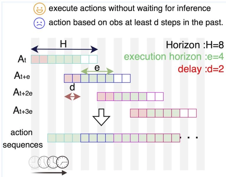
Figure 1: 异步 action chunk 执行示意图。每个执行动作至少基于落后 d 步的 observation，最坏情况会落后 d + e 步。

💡 Figure 1 批读: 这张图基本就是全文的问题陈述。

• H: chunk 总长度
• e: 实际执行多少步之后再请求新 chunk
• d: 推理延迟

一旦 d 和 e 同时变大，机器人执行的就不是“刚刚看到世界之后做出的动作”，而是“基于过去世界快照生成的计划残片”。A2C2 后面所有设计，都是围绕着怎么把这个 stale feedback 问题补回来。

Conventional approaches attempt to mitigate the latency of large models through action chunking (Zhao et al., 2023; Black et al., 2024). By predicting long sequences of actions at once, these methods reduce the frequency of expensive inference calls. However, the chunking strategies can impact performance; robots may experience waiting time during inference, and inconsistencies can arise between successive chunks (Liu et al., 2025). To address this, SmolVLA (Shukor et al., 2025) introduces synchronous execution of the policy, and Real Time Chunking (RTC) (Black et al., 2025) ensures smoother continuity between chunks under asynchrony for diffusion-based action generation. However, these methods still assume that the model predicts fixed-length horizons, which means reactivity to new sensory input remains limited.

Another line of work adopts hierarchical architectures inspired by dual-system reasoning (Kahneman, 2011). Large models serve as a high-level planner (System 2), while smaller policies act as fast executors (System 1). Examples include Hi Robot (Shi et al., 2025), which combines a VLM at the high level with a VLA at the low level, and GR00T-N1 (NVIDIA et al., 2025), which uses a compact policy to refine continuous action chunks. However, since the low-level executor has to wait for predictions from the high-level model, the latency still persists. Consequently, while chunking and hierarchical approaches alleviate some issues, they do not fundamentally solve the challenge of maintaining responsiveness to new observations under the inference delays inherent to VLAs with a large number of parameters.

💡 已有方案为什么不够:

• action chunking: 省的是推理次数，但没解决 chunk 执行期间越来越看不见新 observation 的问题
• RTC: 修的是 inter-chunk continuity，避免新旧 chunk 切换时打架，但是在推理时使用的都是推理起点的observation
• 层级架构: 把大模型当 planner、小模型当 executor，但如果低层仍要等高层结果，延迟依然在

所以 A2C2 的切入点不是“再做一个更平滑的 chunk stitching”，而是把 step-level feedback 单独拿出来补。

To mitigate this problem, in this paper, we propose Asynchronous Action Chunk Correction (A2C2), which is a lightweight correction head that can be executed at every timestep to complement the outputs of large VLA models. Unlike conventional approaches such as action chunking and asynchronous inference, our method introduces a lower-level correction layer that directly integrates the most recent observation referring to the action chunks that high-level model outputs. This correction head does not compete with base (high-level) policies like diffusion- or VLA-based chunk generators; instead, it enhances them by injecting real-time feedback to maintain responsiveness under inference delays and long horizons. Through this design, the proposed framework achieves robustness against dynamic environmental changes and external disturbances, thereby mitigating the critical latency bottleneck in deploying large-scale VLA models for real-time robotic control.

In our experiments on the Kinetix tasks, we measure a 35% point increase in success rate over naive execution and 23% point increase over RTC in the presence of delay. For long execution horizons, we measure a 12% point success rate increase over naive execution and 7% point increase over RTC.

In summary, the contributions of this work are as follows:

• We first formulated delays in policy inference with VLAs that generate action chunks.
• A lightweight add-on action correction policy (A2C2) is introduced to improve reactivity, which can be applied to any VLA model independent of the underlying architecture.
• The method showed substantial improvements in success rates on dynamic tasks and robot manipulation benchmarks with varied inference delays.

💡 A2C2 的定位与贡献:

• 它不是替代 base policy，而是给 base chunk 加一个逐步 residual correction 层
• 它不和 diffusion policy、VLA、RTC 这些路线竞争，而是往它们上面再补一层实时反馈
• 作者先给出延迟形式化，再给出 plug-in 校正头，最后用 Kinetix 和 LIBERO 证明这件事在动态任务和真实 VLA 设置下都成立

🔖 Section 总结

核心洞察

1. 问题不只是推理慢: action chunk 一旦开始执行，就会天然失去对新 observation 的持续利用。
2. RTC 和 A2C2 解决的不是同一个层级: RTC 修 chunk 切换，A2C2 修 chunk 内反应性。
3. A2C2 的出发点很直接: 把大模型保留在 chunk 级规划，把小模型拉回 step 级反应。

2 Problem Formulation

📌 预览

这一节给出全文最重要的形式化：chunk 长度 H、执行 horizon e、推理延迟 d，以及三者之间的可行区间。如果这组符号关系没看懂，后面的方法、实验和 A2C2 的定位都会显得很飘。

We consider an action chunk execution with an imitation learning (IL) policy. As illustrated in Figure 1, an action chunk $A_t = \{a_t, \ldots, a_{t + H - 1}\}$ is from IL policy $\pi$ based on the observation $o_t$ and a language instruction $l$. $H$ is the horizon length, the training sequence length of the IL model $\pi$. We assume it uses $e$ steps of the action chunk, and define it as the execution horizon. Policy predicts the action chunk every $e$ steps as follows:

$$A_t = \{a_t, \ldots, a_{t + H - 1}\} = \pi(o_t, l).$$

💡 Chunk 定义 批读:

• H 决定单次推理吐出多少动作
• e 决定当前 chunk 会被执行多久之后才请求下一个 chunk
• H 偏大时，单次推理更划算，但单个 chunk 更像 open-loop 计划

这一步其实是在给全文立坐标系：后面所有“实时性”讨论，都是围绕一个 H 长度的 chunk 怎么被异步消费展开的。

Also, there is an inference latency. We define the delay $d$ as the number of control steps between receiving an observation $o_t$ and obtaining the corresponding action chunk $A_t$. Formally, it is computed as

$$d = \left\lfloor \frac{\delta}{\Delta t} \right\rfloor,$$

where $\delta$ represents the combined inference and communication time, and $\Delta t$ denotes the duration of a single control step.

💡 Delay 定义 批读:

• 作者把 模型推理时间 和 通信时间 统一压进 d
• 所以这里分析的不只是“本地 GPU 太慢”，也包括真实部署里常见的 client-server VLA 场景
• d 一旦用控制步数而不是秒来表达，后面讨论等待时间、chunk 用尽和 stale observation 都会非常直观

To control delayed, chunked action execution, the agent executes one action per step till a new chunk arrives asynchronously. Additionally, we assume that the policy server can handle only one inference at a time. If the execution horizon $e$ is shorter than the delay $d$, there will be no action during the model inference, which leads to waiting time. On the other hand, if the execution horizon $e$ is longer than $H - d$, there is no action remaining during the inference time. Therefore, the execution horizon $e$ needs to satisfy $d \leq e \leq H - d$.

In this setting, the agent needs to use the actions that are always based on past observations. Each executed action corresponds to an observation at least $d$ steps old. And in the worst case, the agent may need to execute an action that is generated from the $d + e$ steps past observations.

💡 可行区间与真正问题:

• e < d 会出现动作断档，机器人只能等
• e > H - d 会导致推理期间 chunk 用完
• 即使系统工作在合法区间内，执行动作仍然一定是 stale action

所以这节最关键的不是不等式本身，而是它正式说明了：异步 chunk 执行天然会让 action 落后于 observation。A2C2 要修的对象不是“让大模型更快”，而是“让最终执行动作别完全受制于旧 observation”。

🔖 小结

核心洞察

1. H / e / d 是全文坐标系: H 管 chunk 长度，e 管消费速度，d 管推理与通信滞后。
2. 可行执行本身就有硬约束: e 既不能小于 d，也不能大于 H - d，否则系统不是等待就是断粮。
3. 合法不代表闭环: 即使 d ≤ e ≤ H - d，执行动作依然至少落后 d 步，最坏会落后 d + e 步。

3 Method

📌 预览

这是全文核心。A2C2 的方法论很清楚: base policy 继续负责生成 chunk，correction head 只负责在执行阶段逐步做 residual correction。前半节解释 online correction 怎么接入，后半节解释 residual head 怎么训练。

3.1 Overview

We extend the action chunk-based policy $\pi$ by Asynchronous Action Chunking Correction (A2C2), introducing a lightweight correction head $\pi_{a2c2}$ that refines each action within a predicted chunk using the most recent observation, features of the base policy, and a temporal position feature. This framework enables step-wise online correction without retraining the base policy and is complementary to methods such as RTC (Black et al., 2025).

💡 方法的角色分工:

• base policy: 继续生成 chunk，保留大模型能力
• correction head: 每步纠偏，专门看最新 observation

所以 A2C2 不是替代 base policy，而是把“规划”和“闭环修正”拆成两个时间尺度。

At time $t$, observation $o_t$ is sent to the policy server. Then, the base policy $\pi$ generates the action chunk $A_t = \{ a_t^{\mathrm{base}}, \dots, a_{t + H - 1}^{\mathrm{base}} \}$ within inference delay $d$ as

$$A_t = \{ a_t^{\mathrm{base}}, \ldots, a_{t + H - 1}^{\mathrm{base}} \} = \pi(o_t, l).$$

💡 Base Chunk 批读:

• A2C2 并不改变 base policy 的 chunk 生成方式
• 大模型依然负责给出一个完整的 chunk 主干
• 这也是它能作为 plug-in 模块接到现有 VLA / diffusion / flow policy 上的前提

Subsequently, at time $t + k$ ($d \leq k \leq d + e$), time feature $\tau_k$, base action $a_{t + k}^{\mathrm{base}}$, latest observation $o_{t + k}$, base policy latest representation $z_{t + k}$, and language instruction $l$ are added to the correction head $\pi_{a2c2}$. The positional feature $\tau_k$ is represented by a sinusoidal embedding that provides periodic structure over the chunk length $(\sin(2 \pi \frac{k}{H}), \cos(2 \pi \frac{k}{H}))$. The correction head integrates this information and predicts the residual action $\Delta a_{t + k}$ as

$$\Delta a_{t + k} = \pi_{a2c2}(o_{t + k}, a_{t + k}^{\mathrm{base}}, \tau_k, z_{t + k}, l).$$

💡 Residual Prediction 批读:

• 该式表示：correction head 在时刻 $t+k$ 基于最新观测、base action、时间位置与任务上下文，预测一个残差项 $\Delta a_{t+k}$，用于对当前将执行的动作做局部修正。
• $\Delta a_{t+k}$ 是在时刻 $t+k$ 对 base action 的残差修正，因此 correction head 预测的不是整段新动作，而是当前执行步的增量。
• $o_{t+k}$ 是执行时刻 $t+k$ 的最新 observation，用于补偿 chunk 生成之后环境状态的变化。
• $a_{t+k}^{\mathrm{base}}$ 是 base policy 为该时刻给出的原始动作，作为 correction 的参照中心，保证修正建立在原有计划之上。
• $\tau_k$ 是 chunk 内位置特征，指示当前修正对应第 $k$ 个 action，使模型区分 chunk 前段、中段和后段的时间语义。
• $z_{t+k}$ 是 base policy 的内部表示，$l$ 是语言指令；二者共同提供任务上下文，约束 correction 不偏离原任务语义。

Figure 2: A2C2 总览。大模型继续产出 chunk，小模型在 chunk 内逐步修正当前动作。

💡 Figure 2 批读: 如果 RTC 是“新旧 chunk 的粘合剂”，A2C2 更像“当前 action 的校准器”。它并不回头重采整个 chunk，而是只修改马上要执行的那个 action。

• 图的下半部分表示：base policy 先基于时刻 $t$ 的 observation 生成一个完整的 action chunk，A2C2 不改变这一步的 chunk-level 规划方式。
• 中间一排方块表示 base chunk 中的各个 action；其中真正进入执行阶段的是从 $t+d$ 开始的一段，而不是整段动作一次性重写。
• 图中的 RP / correction head 表示：当系统执行到 chunk 内第 $k$ 步时，会取出当前的 base action，并结合最新 observation $o_{t+k}$ 与位置特征 $\tau_k$ 预测一个残差项。
• 图的上半部分表示：最终执行的不是原始的 $a_{t+k}^{\mathrm{base}}$，而是修正后的 $a_{t+k}^{\mathrm{exec}} = a_{t+k}^{\mathrm{base}} + \Delta a_{t+k}$。
• 因此，这张图最想强调的是 A2C2 的双时间尺度结构：base policy 负责 chunk-level 主方案，correction head 负责 step-level 局部修正；它修的是当前 action，而不是重写整个 chunk。

The residual action $\Delta a_{t + k}$ is added to the base action $a_{t + k}^{\mathrm{base}}$ and outputs the execution action $a_{t + k}^{\mathrm{exec}}$ as

$$a_{t + k}^{\mathrm{exec}} = a_{t + k}^{\mathrm{base}} + \Delta a_{t + k}.$$

💡 Execution Action 批读:

• 最终执行动作是 base action + residual
• 这种写法把 base policy 的能力默认保留下来，把 correction head 的职责限制在“局部修偏”
• 这也是 A2C2 计算开销小、训练更稳定的重要原因

Base policy $\pi$ infers an action chunk every $e$ steps with $d$ delay. On the other hand, we assume that the model size of the correction head $\pi_{a2c2}$ is small enough to run every step, which means the inference time of the head is smaller than the duration of a single control step $\Delta t$. Refer to Figure 2 for the overview.

Our method differs from existing approaches for asynchronous inference in the following aspects:

• Time-aware correction: The correction head explicitly conditions on the position within the action chunking VLA using a temporal feature.
• Chunk-level smoothness: By specifying which element of the chunk is being corrected, the method produces smoother corrections across horizons.
• Data compatibility: Training uses the same demonstration datasets as the base VLA policy, which does not require reinforcement learning fine-tuning.
• Real-time feedback: New observations are always incorporated, improving robustness under inference delay in dynamic tasks.

💡 这四点里最关键的是最后一点: A2C2 真正恢复的是 实时反馈链路。其余设计都是为了让这个反馈既稳定又能和 base chunk 对齐。

3.2 Model Training Procedure

First, we train the base policy $\pi$ with the dataset

$$\mathcal{D}_{\mathrm{base}} = \left\{ \left\{ \{o_t, a_t\}_{t=0 \ldots T_n}^{\,n}, l^n \right\}_{n=1 \ldots N} \right\},$$

💡 Base Dataset 批读:

• 第一阶段仍然是普通的 imitation learning 数据：observation、action 和 language instruction，先沿用 base policy 原本的数据形态

where $N$ denotes the number of episodes in the dataset. Afterward, we add the output action chunk $\hat{A}_t$ of the inference from base policy $\pi$ for each step in the dataset $D_{\mathrm{base}}$ as

$$\hat{A}_t = \{\hat{a}_t, \ldots, \hat{a}_{t + H - 1}\} = \pi(o_t, l).$$

💡 Predicted Chunk 批读:

• 第二阶段先让 base policy 在数据上离线跑一遍
• 这样 correction head 训练时看到的不是理想 expert chunk，而是 base policy 实际会吐出来的 chunk
• 这是后面 residual 学习成立的关键，因为它学的是“expert 相对 base 输出差多少”

With these inference results, we created a new dataset for correction head training $D_{\mathrm{cor}}$ as

复杂数据集定义：correction head 的训练样本显式包含历史时刻预测出的 base action 与时间特征。

💡 Correction Dataset 批读:

• 这一步是在 $\mathcal{D}_{\mathrm{base}}$ 的基础上，为每个时刻补上 base policy 实际预测出来的 chunk 信息，从而构造 correction head 的训练样本。
• 其中 $\hat{a}_{t-k}^{k}$ 表示：在时刻 $t-k$ 基于当时 observation 预测出的 chunk 中，第 $k$ 个位置对应的 base action；它正对应了执行到时刻 $t$ 时将要被修正的那个动作。
• 因此，$\mathcal{D}_{\mathrm{cor}}$ 的核心作用是把训练输入改写成测试时的真实形式：当前 observation、chunk 内位置以及 base policy 给出的原始动作共同决定 correction，而不是直接从 observation 重新学习一个新 policy。

$\hat{a}_{t-k}^k$ is the $k$-th action in the action chunk inferred by the base policy from the observation at time $t-k$. Then, the correction head $\pi_{a2c2}$ is trained to predict the residual action, i.e., the difference between the target action and the base policy output. The target action is the action in the dataset that was originally collected from expert demonstrations. Formally, given the target action $a_{\mathrm{target}}$ and the base policy output $a_{\mathrm{base}}$, the residual target is defined as

$$\Delta a_{\mathrm{residual}} = a - \hat{a}.$$

$\hat{a}$ is a base action inferred by the base policy. There are some possible combinations of the base action with different time features $\tau$. The predicted residual action is denoted by $\Delta a_{\mathrm{residual}}$. The loss function is the mean squared error (MSE):

复杂损失定义：correction head 只学 residual，不需要重新学习整条动作序列。

Where $N$ denotes the batch size, i.e., the number of training samples in a mini-batch.

💡 Residual Target&MSE Loss 批读:

• 训练目标直接拟合 $a - \hat{a}$，监督的仍然是 residual，而不是最终 action 本身
• 所以 loss 的语义很直接：只要 correction head 把“expert 相对 base 的偏差”学准，它就完成任务了
• 默认承认 base policy 已经会做大部分事情，correction head 只负责补最后那点由 stale observation 带来的误差

🔖 Section 总结

核心洞察

1. 推理时分工明确: base chunk 负责“主计划”，correction head 负责“每步纠偏”。
2. 训练时只学残差: correction head 学的是 expert action 相对 base action 的偏差，不是重学整条策略。
3. 系统设计足够克制: A2C2 不回头重采 chunk，而是在现有 chunk 上做局部、低成本、实时的闭环修正。

4 Experimental Setup

📌 预览

这一节回答两个问题：A2C2 在什么任务上测，correction head 具体做成什么样。Kinetix 用来测高动态与延迟鲁棒性，LIBERO Spatial 用来测标准 manipulation 和 long-horizon 退化；两者一起构成“低维高动态”到“多模态 VLA”两端的验证。

4.1 Benchmark and Datasets

We use the two simulation environments, Kinetix and LIBERO Spatial, for the experiments. Kinetix is first used for evaluating the performance under highly dynamic manipulation and locomotion tasks. Secondly, we used the LIBERO Spatial benchmark to evaluate the performance as a standard benchmark of robot manipulation. Especially, because Shukor et al. (2025) reports that long-horizon significantly degrades performance in LIBERO Spatial, making the task a natural choice for evaluating robustness under long horizons.

4.1.1 Kinetix

We used Kinetix, which provides demonstrations across 12 highly dynamic tasks (see Appendix A.1). It includes environments ranging from locomotion and grasping to game-like settings. Importantly for our setting, Kinetix contains highly dynamic environments where delayed or inconsistent action generation quickly leads to failure. This makes it a natural testbed for studying the limitations of action chunking and for benchmarking inference-time algorithms such as RTC, which aim to preserve responsiveness and continuity under latency.

Unlike quasi-static benchmarks, Kinetix environments employ torque- and force-based actuation, making asynchronous inference crucial. Kinetix consists of 12 tasks without language input. One million steps of data were collected by using an expert model. Following RTC experiments, we first train expert policies using RPO (Rahman & Xue, 2022) and a binary success reward. For each environment, a 1-million transition dataset is generated with the expert policy.

💡 为什么先上 Kinetix: 如果任务本身是 quasi-static，很多 stale action 问题不会立刻暴露。Kinetix 的价值就在于它对时序错位极其敏感。

4.1.2 LIBERO

LIBERO is a benchmark suite designed to study lifelong robot learning with a focus on knowledge transfer across tasks (Liu et al., 2023). They offer several task suites and datasets. In this work, we specifically use the LIBERO Spatial dataset, which emphasizes spatial reasoning in manipulation tasks as a widely used benchmark for robot manipulation.

For benchmarking 3D robot manipulation, we used the LIBERO Spatial benchmark, which provides 432 episodes and 52,970 frames across 10 tasks. The dataset consists of multimodal input, including top and wrist RGB images (256 × 256), an 8-dimensional state, and language instructions.

💡 为什么还要测 LIBERO: 这能证明 A2C2 不是只适合无语言、低维状态的 toy setting，而是也能接到真正的 VLA 输入形态上。

4.2 Model Training

In Kinetix, we used a flow-matching policy as the base model, following prior work on RTC (Black et al., 2025). The correction head network is a 3-layer multilayer perceptron (MLP). The input layer receives the concatenation of the state vector (2722-dim), the base action (6-dim), and the 2-dimensional sinusoidal positional feature. We did not use language instructions or latent representations from base policies, as the model was trained and evaluated separately for each task. Hidden layers have 512 units each with ReLU activation (Nair & Hinton, 2010) and layer normalization (Ba et al., 2016). The output layer produces a 6-dimensional residual vector, which is added elementwise to the base action. The total parameter count is 0.31M. Figure 3 shows the implementation detail for the Kinetix experiment.

Figure 3: Kinetix 中的 correction head 是一个很小的 MLP，输入当前状态、base action 和 chunk 位置编码，输出 residual action。

💡 Figure 3 批读:

• Kinetix 版本里，计算 $\Delta a_{t+k}$ 的结构就是一个很小的 $3$ 层 MLP。
• 输入端直接拼接三类信息：当前状态 $s_{t+k}$、原始动作 $a_{t+k}^{\mathrm{base}}$ 和时间位置特征 $\tau_k$；这里没有额外的视觉、语言或 latent 融合模块。
• 中间层只是标准的全连接变换，因此这个版本本质上是在测试：仅靠当前状态与 base action，是否已经足以恢复 step-level reactivity。
• 输出端给出一个与 action 维度相同的残差向量 $\Delta a_{t+k}$，再与 $a_{t+k}^{\mathrm{base}}$ 逐元素相加得到执行动作。
• 这张图强调的是最小实现：作者有意把 correction head 压到 $0.31\mathrm{M}$ 参数，说明 A2C2 的核心并不依赖复杂结构，而在于“每步做残差修正”这一机制本身。
• 这里作者刻意用最小设计验证观点。如果只靠 state + base action + time feature 就能显著提分，说明问题确实出在 step-level reactivity，而不是必须上更复杂的 world model。

For LIBERO Spatial, we adopted SmolVLA (Shukor et al., 2025) (450M parameters) as the base, since it provides competitive performance among VLA models. The correction head consists of a transformer encoder and a lightweight MLP. Visual observations (top and wrist cameras) are encoded into 512-dimensional tokens using a ResNet-18 (He et al., 2016) pretrained on ImageNet (Deng et al., 2009). Language instructions are embedded by the smolVLM encoder provided in the base policy. The base action, latent features of the base policy, and the sinusoidal time embedding are also projected into 512-dim tokens. All tokens are concatenated and processed by a 6-layer transformer encoder. The pooled embedding, along with the base action and state vector, is passed through a 3-layer MLP (hidden size 512) to predict the residual action. The number of total parameters is 32M. Figure 4 shows the implementation detail for the LIBERO experiment.

Figure 4: LIBERO 中的 correction head 更复杂，需要消费视觉 token、语言特征、state、base action 和时间嵌入。

💡 Figure 4 批读:

• LIBERO 版本里，计算 $\Delta a_{t+k}$ 的结构不再是单纯的 MLP，而是“transformer encoder $+$ lightweight MLP”的两段式结构。
• 输入端先把视觉观测、语言特征、base latent、base action 和时间特征都投影成 token，再交给 transformer encoder 做多模态融合；这一步负责回答“当前视觉局面和任务语义下，这个 base action 是否需要改”。
• transformer 的 pooled embedding 随后与 $a_{t+k}^{\mathrm{base}}$ 和状态向量一起送入一个 $3$ 层 MLP，最终输出残差 $\Delta a_{t+k}$。
• 因此，Kinetix 版本更像是状态驱动的局部修正器，而 LIBERO 版本已经是多模态条件化的 step-level correction head。

We also release the source code for both Kinetix and LIBERO experiments. See Appendix A.3 for the details.

🔖 Section 总结

核心洞察

1. Benchmark 设计有明确分工: Kinetix 负责放大延迟和动态性问题，LIBERO Spatial 负责验证多模态 VLA 场景下是否仍然成立。
2. 两套 correction head 是按输入复杂度扩展的: Kinetix 用最小 MLP 验证思想，LIBERO 再把视觉、语言和 latent 一起接进来。
3. 作者始终坚持“小头补反馈”: 不管在哪个 benchmark 上，correction head 都被刻意控制在显著小于 base model 的规模。

5 Results

📌 预览

这一节直接检验论文 claim: A2C2 是否真的比 naive async 和 RTC 更稳。关键信号有两个: 随着 delay 增大它掉得更慢；即使 delay = 0，只要 horizon 变长它也仍然有收益。

5.1 Kinetix

We evaluate the proposed action chunk correction framework in the Kinetix benchmark under varying inference delays $d$ and execution horizons $e$. Figure 5 reports success rates aggregated across all 12 tasks. There are two baseline comparisons. First is Naive async. This strategy does not pay attention to the previous action chunk at all when generating a new one, naively switching chunks as soon as the new one is ready. Second is RTC. As expected, both the naive async and RTC baselines degrade significantly as either the delay $d$ increases or the horizon $H$ becomes longer. In particular, when $d \geq 3$, the naive baseline suffers a sharp drop in success rate due to compounding errors from executing outdated action chunks. RTC inference partially mitigates this issue by overlapping prediction and execution, but performance still declines as the execution horizon increases.

In contrast, the action chunk correction maintains consistently higher success rates across all settings. Because it refines each action using the most recent observation, the action chunk correction can counteract both the temporal misalignment introduced by inference delay and the drift that accumulates within long action horizons. For example, at delay $d = 4$, our proposed method achieves nearly 35% higher success than the naive baseline, and remains above 85% even for horizons $H = 7$. This demonstrates that real-time correction of action chunks maintains performance both with inference delays and with long-horizon execution.

Figure 5: Kinetix 总结果。左图固定 e = max(d, 1) 看 delay 效应，右图固定 d = 1 看 execution horizon 效应。

💡 Figure 5 批读:

• 左图 说明 A2C2 对显式推理延迟更稳
• 右图 说明 A2C2 对长 horizon 带来的 chunk 内漂移也更稳
• RTC 通常比 naive 好，但 A2C2 整体抬高了曲线下界

5.2 LIBERO Spatial

Figure 6 and Table 1 summarize the evaluation on the LIBERO Spatial benchmark. We tested the Naive async and A2C2 on this setting. Across 10 manipulation tasks with multimodal inputs, the correction head consistently improved success rates over the naive baseline under both long horizons and injected delays. For example, with execution horizon $H = 40$ and delay $d = 10$, the naive baseline achieved only 67% success, whereas A2C2 reached 84%. Even when no delay was present, action chunk correction provided notable gains at long horizons ($H = 50$, $d = 0$), raising success from 72.2% to 81.6%. These results demonstrate that residual refinement by the correction head mitigates the degradation caused by outdated action chunks and restores closed-loop responsiveness, enabling large VLA models to maintain high success rates in tasks that require fine-grained spatial reasoning.

Figure 6: LIBERO Spatial 结果。左图固定 execution horizon 看 delay 效应，右图固定 d = 0 看 execution horizon 效应。

💡 Figure 6 批读:

• 这里已经不是低维状态控制，而是多模态 VLA 设置，所以结果比 Kinetix 更接近“真实大模型部署”场景
• 左图说明即使 base policy 变成 SmolVLA，A2C2 仍然能对抗显式 delay
• 右图说明即使没有注入 delay，随着 horizon 变长，A2C2 仍然能持续提分，这再次证明它修的是 chunk 执行期的 open-loop 缺口

Table 1: LIBERO Spatial success rate. 50 rollouts per task.

💡 Table 1 批读:

Method	Execution Horizon e	Delay d	Success Rate (%)
Naive	10	0	81.8
A2C2 (Ours)	10	0	89.2
Naive	40	10	64.4
A2C2 (Ours)	40	10	84.2
Naive	50	0	72.2
A2C2 (Ours)	50	0	81.6

e = 50, d = 0 这一行提升很大，说明它修补的不只是通信/推理延迟，还包括 chunk 自身越来越 open-loop 的问题

🔖 Section 总结

核心洞察

1. Kinetix 结果证明两件事: delay 上升时 A2C2 更稳，horizon 变长时 A2C2 也更稳。
2. LIBERO 结果把结论推进到真正 VLA 场景: 多模态输入下它依然能提升成功率，不只是低维控制里的技巧。
3. 最关键的证据是 zero-delay long-horizon 仍能提分: 这说明 A2C2 修的是更一般的 step-level closed-loop feedback 缺口。

6 Related Work

📌 预览

Related Work 覆盖了 3 条主线：chunk-based imitation learning / VLA、异步 chunk 执行、减少推理延迟。A2C2 的独特定位是：它不重做 chunk stitching，也不只追求把模型变快，而是给现有 chunk-based policy 增加一个 step-level correction layer。

Imitation learning and VLAs: Imitation learning (IL) trains agents from demonstrations provided by humans or expert policies, and has been a representative approach in learning robotic control (Osa et al., 2018). Recent advances have introduced generative sequence models to improve consistency and scalability. Diffusion Policy (Chi et al., 2023) utilizes diffusion models for action generation, enabling it to handle the multimodality of data distribution in imitation learning. In parallel, the Action Chunking Transformer (ACT) (Zhao et al., 2023) proposes a transformer-based policy that outputs action chunks rather than single-step actions, producing coherent behaviors while enabling faster inference. In addition, flow-based approaches, such as Flow Policy (Zhang et al., 2024), generate actions by learning continuous transport maps instead of iterative denoising.

Building on these foundations, a new class of vision-language-action (VLA) foundation models has emerged (Kawaharazuka et al., 2024), including $\pi_0$ (Black et al., 2024), OpenVLA (Kim et al., 2024), GR00T (NVIDIA et al., 2025), and SmolVLA (Shukor et al., 2025). These models adopt chunk-based prediction as the de facto standard for inference, similar to ACT (Zhao et al., 2023). Vision-language-action (VLA) models achieve broad task generalization by aligning multimodal inputs, but their architectures are considerably larger than diffusion- or transformer-based imitation policies. For instance, $\pi_0$ has about 3B parameters and OpenVLA around 7B, which makes inference latency significant even on modern GPU-accelerated hardware. While these models demonstrate the promise of scaling and multimodal grounding, their computational footprint exacerbates the latency problem in real-time control.

💡 Chunk-based VLA 生态梳理:

• 生成策略主线: IL 里的 action generation 已经从单步预测走向 action chunking，代表路线包括 ACT、Diffusion Policy、Flow Policy
• VLA 扩展: 这些 chunk-based 生成范式进一步被扩展到 VLA，形成 $\pi_0$、OpenVLA、GR00T、SmolVLA 这类大模型机器人策略
• 共同前提: 这些方法默认接受一个现实交换条件: 用 chunk 换更少的推理次数，但执行阶段也更容易变 open-loop
• A2C2 的位置: 它不替换 chunk-based policy，而是在这个既定前提上补一个逐步 correction 头，让 chunk 执行时重新看见最新 observation

Asynchronous chunk execution: As model sizes increase, inference latency becomes a significant bottleneck, motivating asynchronous policy frameworks. In particular, SmolVLA (Shukor et al., 2025) proposed a server-client architecture for mitigating inference delays. In this setup, the server receives observations and performs inference with a delay of $d$ control steps (including communication latency), then transmits an action chunk of horizon $H$ to the client. Then, the client executes these actions sequentially. However, because the $d$ delayed actions are not yet available at execution time, the client continues executing actions from the previous chunk until the new chunk arrives. This design ensures continuity but introduces the risk of inconsistency between consecutive chunks. For example, the earlier chunk may predict avoiding an obstacle by moving left, while the newly received chunk may instead suggest moving right. Such mismatches across chunks can cause jerky motion and noticeable performance degradation, especially in dynamic environments.

To fix the chunk mismatches, Real Time Chunking (RTC) (Black et al., 2025) is proposed. It is an inference-time algorithm that enables smooth asynchronous execution for action-chunking policies by posing chunk switching as an inpainting problem. Specifically, it generates the next action chunk while executing the current one, freezing actions guaranteed to execute and inpainting the rest.

💡 异步执行路线对比:

• SmolVLA server-client 架构: 先把“大模型推理有延迟”这件事系统化，明确 client 需要在旧 chunk 上继续执行，直到新 chunk 到达
• RTC: 重点解决 inter-chunk continuity，也就是新旧 chunk 切换时不要打架
• A2C2: 重点解决 intra-chunk reactivity，也就是当前正在执行的 action 能不能根据最新 observation 及时修正
• 两者关系: RTC 更像 chunk stitching，A2C2 更像 per-step calibration；它们不是互斥方案，而是可以叠加的两层补丁

Reducing inference latency: One natural way to enhance a model’s real-time performance is to reduce its inference time. Streaming Diffusion Policy (Høeg et al., 2024) or Streaming Flow Policy (Jiang et al., 2025) presents a new training procedure that enables faster inference. More generally, optimizations such as model compression (Lin et al., 2024) or memory optimization (Kwon et al., 2023) of models can also improve inference speed. However, as long as model scale and communication overhead prevent action generation from being faster than the control step, the challenges highlighted in this work remain unresolved.

💡 加速推理路线的局限:

• Streaming Diffusion Policy、Streaming Flow Policy、模型压缩、内存优化，目标都是把推理做得更快
• 这条线当然重要，但它默认的解法仍然是“尽量缩短前向时间”
• A2C2 的论点更强一些：只要单次前向传播仍慢于 control step，系统里就需要一个能在 step 级反应的补偿模块
• 所以 A2C2 和加速路线是正交的：你可以先把模型加速，再用 A2C2 处理剩余的实时性缺口

🔖 Section 总结

A2C2 的定位

Chunk-based IL / VLA
    ↓ 已经很强，但执行期越来越 open-loop
异步执行 (SmolVLA server-client, RTC)
    ↓ RTC 修的是 chunk 切换连续性
减少推理延迟 (streaming / compression / optimization)
    ↓ 仍未必快到每个 control step 都能重跑大模型
A2C2
    → 在 chunk 内增加 step-level correction
    → 用小头补最新 observation 反馈
    → 与 RTC / 加速路线正交，可叠加

7 Conclusion

📌 预览

结论部分回收全文主张：A2C2 是一个轻量、可插拔、与 base VLA 正交的 correction mechanism。作者最后真正想落下来的，不只是“这个方法在 benchmark 上有效”，而是“未来更大的 VLA 很可能需要显式的 step-level correction 才能现实部署”。

In this paper, we propose Asynchronous Action Chunk Correction (A2C2), which introduces a lightweight action correction head by augmenting a large base policy, such as VLAs. A2C2 addresses the challenge of preserving reactivity under inference delays and long execution horizons of action chunking policies. The correction head is trained on the same dataset as the base policy and, in principle, can be added to any off-the-shelf VLAs. Our experiments in both the Kinetix simulation suite and the LIBERO Spatial benchmark demonstrated that Asynchronous Action Chunk Correction (A2C2) consistently maintained high success rates, even in settings where naive or RTC degraded significantly.

While our approach adds minimal overhead compared to full model inference, further work is needed to validate its scalability to richer language instructions, out-of-distribution settings, and more dynamic tasks beyond those in LIBERO Spatial. Addressing these challenges would broaden the applicability of action chunk correction and strengthen its role as a general mechanism for enhancing reactivity in large policy architectures.

💡 定位与局限性:

• 作者先把最核心的 claim 再收一遍：A2C2 解决的是 action chunking policy 在 delay 和 long horizon 下的反应性损失
• 它的工程定位依然很克制：轻量、可插拔、沿用 base policy 数据、不要求重训大模型
• 这里其实是在强调，A2C2 最有吸引力的地方不是“提出了一个新大模型”，而是“用一个很小的附加模块解决了一个会越来越普遍的问题”
• richer language、OOD、以及比 LIBERO 更动态的任务，仍然需要进一步验证

Recently, Large Language Models (LLMs) and Vision-Language Models (VLMs) have demonstrated improved generality through parameter scaling, as established by neural scaling laws (Kaplan et al., 2020). Since recent VLA policies are built upon these models, it is reasonable to expect that future VLAs will continue to grow in size to support deployment across diverse environments and tasks. Our work can be viewed as a step toward enabling such scaled VLAs to operate in real time without sacrificing responsiveness by introducing a lightweight correction mechanism that mitigates the effects of inference latency.

Moreover, inference of models with billions of parameters already exceeds the computational capacity of on-board processors on most robotic platforms. In practice, this motivates client-server architectures where the VLA runs on a remote server and the robot queries it over a network. In this setting, by explicitly treating communication delay as part of the inference latency in our formulation, our framework naturally extends to client-server architectures where large VLAs are executed remotely. Thus, our framework provides a pathway to leverage the generalization benefits of large-scale VLAs while still maintaining reactivity in real-world deployments, enabling the design of next-generation VLA systems that combine scalability with responsiveness.

💡 系统层面的真正落点:

• 作者把 scaling law、远程推理、client-server 架构放进结论，不是为了补背景，而是在说明这个问题未来只会更严重
• 如果大模型继续变大、越来越依赖远程 GPU 推理，那么“每个 control step 都重跑大模型”只会越来越不现实
• 在这个意义上，A2C2 想提示的是一种更长期的系统范式：chunk 级规划 + step 级校正

🔖 Section 总结

核心洞察

1. 短期价值很明确: A2C2 是一个对现有 chunking policy 很实用的 plug-in 补丁。
2. 作者承认边界仍然存在: richer language、OOD 和更动态任务还没有被充分覆盖。
3. 长期判断更重要: 未来大模型机器人控制很可能需要显式的双时间尺度结构，也就是 chunk 级规划配合 step 级纠偏。

8 Appendix

📌 预览

Appendix 里最值钱的是三类信息: 任务环境、训练超参数、以及推理时间/硬件成本。正文负责说明 A2C2 为什么有效，这一节负责说明作者到底是怎么把它做出来的。

A.1 Kinetix Simulation Detail

A.1.1 Environment

We reused the 12 tasks from the Kinetix benchmark (Matthews et al., 2025) used in the RTC paper (Black et al., 2025). A sample visualization of each of the environments is shown in Figure 7. The Kinetix environment has an observation space with 2722 dimensions which do not include any images. Instead, it encodes information about polygons, circles, joints, thrusters, gravity, and the states of motors and thrusters described below. For entities not used in a given task, their corresponding entries are zero-padded. The action space has 6 dimensions. The first four correspond to motor controls, and the last two correspond to thruster controls. For unused actuators, their entries are set to zero via padding.

Figure 7: Kinetix 的 12 个任务示意图。

💡 Kinetix 环境特点: 没有图像输入，状态向量很大，但最关键的是物理过程动态性强，所以 stale action 会很快放大成失败。

A.1.2 Dataset Generation and Training Detail

An imitation learning dataset was required to test the flow policy and our correction head. In the Kinetix simulation, we follow the RTC implementation. First, we trained the expert policy with RPO (Rahman & Xue, 2022) on 8 seeds per task for 64 million environment steps each. For each task, we load the best-performing checkpoint for each seed and discard some seeds if they did not reach a certain success threshold. Then, we used the expert model to generate 1 million environment steps for each task. After that, we train the flow policy with the generated dataset. We saved the checkpoints for each, but used the last checkpoint for the evaluation.

💡 Table 2 批读:
Table 2: Kinetix flow policy 的训练超参数。

Hyperparameter	Value
Learning rate	3 x 10^-4
Gradient norm clip	10.0
Weight decay	1 x 10^-2
Warmup steps	1000
Batch size	512
Number of epochs	32

这张表说明 Kinetix 的 base flow policy 训练并不夸张，重点是一个相对标准的 imitation-learning 配置：较大的 batch、固定 warmup、32 个 epoch。A2C2 后面的收益不是靠把 base policy 训练得异常复杂换来的。

💡 Table 3 批读:
Table 3: Kinetix correction head 的训练超参数。

Hyperparameter	Value
Batch size	512
Number of epochs	16
Learning rate	1 x 10^-4
Weight decay	1 x 10^-3
Gradient norm clip	5.0
Warmup steps	500

和 Table 2 对照看，correction head 的训练更短、更轻，学习率和 warmup 也更保守。这很符合它的角色：不是重学整条策略，而是在 base policy 上做第二阶段 residual 校正。

The correction head is then trained with the flow policy. The correction policy requires the base action from the base policy, so at every step, we infer the action chunk from the base policy and use it and the dataset to train the correction head. During the base flow policy training, we used a constant learning rate and added some warmup stage. See Table 2 for more details on the settings. For the correction head training, we used the parameters shown in Table 3. In both the flow policy and A2C2 training, the AdamW optimizer (Loshchilov & Hutter, 2017) was used.

💡 训练成本观察: 在 Kinetix 里，A2C2 的训练流程仍然依赖先把 base policy 训练好，然后再围绕 base action 构造 correction 数据集。这意味着它是一个明确的“第二阶段训练”方案。

A.1.3 Evaluation Details

In the evaluation, we rolled out 2048 per task and computed the success rate for different delays and execution horizon lengths. In the Kinetix simulation, we tested all combinations of delay and execution horizons compatible with the chosen action chunk size. All results are in Table 4.

Table 4: Kinetix 在不同 delay / execution horizon 下的完整结果。每个单元格依次给出 naive、RTC、A2C2。

💡 Table 4 批读:

• 这张表是 Kinetix 的完整结果矩阵：列是 execution horizon e，行是 inference delay d，每个可行单元格按顺序给出 naive / RTC / A2C2
• 最值得看的不是单个格子，而是整体趋势：随着 d 变大、e 变长，naive 先明显崩，RTC 能缓一部分，但 A2C2 基本一直把成功率维持在更高的平台
• 例如在最困难的几组条件里，naive 和 RTC 已经掉到 50% 到 70% 左右时，A2C2 仍然大多维持在 86% 到 87% 一带，这说明它补的不是边缘收益，而是系统性的 step-level feedback
• 表里空白的位置也不是漏实验，而是因为那些 d / e 组合本身不满足前面 problem formulation 里的可行约束

A.2 LIBERO Simulation Detail

A.2.1 Environment

LIBERO Spatial consists of 10 tasks. We evaluated all tasks, and the corresponding language instructions are listed below. The language instructions are:

1. pick up the black bowl between the plate and the ramekin and place it on the plate
2. pick up the black bowl next to the ramekin and place it on the plate
3. pick up the black bowl from the table center and place it on the plate
4. pick up the black bowl on the cookie box and place it on the plate
5. pick up the black bowl in the top drawer of the wooden cabinet and place it on the plate
6. pick up the black bowl on the ramekin and place it on the plate
7. pick up the black bowl next to the cookie box and place it on the plate
8. pick up the black bowl on the stove and place it on the plate
9. pick up the black bowl next to the plate and place it on the plate
10. pick up the black bowl on the wooden cabinet and place it on the plate

💡 这里能看出 LIBERO 的作用: 任务虽然都围绕一个 object family，但输入已经包含语言和视觉，所以比 Kinetix 更接近真实 VLA 设置。

A.2.2 Dataset and Training Detail

We used the LIBERO dataset with the LeRobot dataset format available on Hugging Face and used the LeRobot framework to read the dataset. LeRobot also has a well-organized training pipeline and makes it easy to create and try new architectures.

First, we trained SmolVLA as a base policy. There is an option for training the policy from scratch or fine-tuning the pretrained model. In our setting, we chose training from scratch because SmolVLA is pretrained mainly with S0-101, which is a different embodiment from the Franka arm used in the LIBERO benchmark.

In the Kinetix simulation, the base policy predicts the action chunk every time in correction head training. However, this is too time-consuming with a large VLA model. Then, we added the inference result of SmolVLA on the dataset for training the correction head. The new dataset has all the LIBERO Spatial data, the action chunk result, and the VLM latent representation from the SmolVLA policy for each step.

After that, we trained the correction head with the dataset we created. For SmolVLA training, we trained a model from scratch with a cosine learning scheduler, which is the default setting for SmolVLA training. The parameters for SmolVLA training are in Table 5.

For correction head training, we use a constant learning rate of 1e-5. High learning rates, such as 1e-4, do not work well for correction head training. See Table 6.

In both SmolVLA and correction head training, the AdamW optimizer was used (Loshchilov & Hutter, 2017).

💡 Table 5 批读:
Table 5: LIBERO 上 SmolVLA 的训练超参数。

Hyperparameter	Value
Learning rate	1 x 10^-4
Scheduler	Cosine
Warmup steps	1000
Decay steps	30000
Minimum learning rate	2.5 x 10^-6
Batch size	64
Training steps	100000
Optimizer epsilon	1 x 10^-8
Optimizer weight decay	1 x 10^-10
Gradient norm clip	10

Cosine scheduler、10 万步训练、较小 batch size，说明 LIBERO 这边的 base policy 成本远高于 Kinetix。

💡 Table 6 批读:
Table 6: LIBERO correction head 的训练超参数。

Hyperparameter	Value
Learning rate	1 x 10^-5 (constant)
Batch size	64
Training steps	200000
Optimizer weight decay	1 x 10^-5
Model dimension	512
Number of heads	8
Number of encoder layers	6

这张表和 Table 5 必须对照着看。SmolVLA 用的是标准的大模型训练配方，而 correction head 这里最醒目的信息是学习率被压到 1e-5 且保持 constant。作者正文也明确说了 1e-4 不行，这说明多模态 correction head 对优化稳定性更敏感。
在真正的大 VLA 上，作者不再每步都实时跑 base model 生成训练监督，而是先离线缓存 SmolVLA 的 chunk 与 latent，再训练 correction head。这是工程上必须做的折中。

A.2.3 Evaluation Detail

For the evaluation, we tested various combinations of delay steps and horizon steps first. We tested 10 rollouts per task, and LIBERO Spatial has 10 tasks. Then, to evaluate more precisely, we selected 3 pairs of delay and horizon, (0, 10), (10, 40), (0, 50), and rolled out 50 episodes per task. All results for LIBERO Spatial are shown in Table 7.

💡 Table 7 批读:
Table 7: LIBERO Spatial 在不同 execution horizon / delay 组合下的完整结果。

Execution Horizon e	Inference Delay d	Naive	A2C2 (Ours)
40	10	0.67	0.84
40	5	0.66	0.86
40	3	0.65	0.86
40	1	0.74	0.83
10	10	0.75	0.88
10	5	0.82	0.92
10	3	0.81	0.89
10	1	0.83	0.92
50	0	0.71	0.84
40	0	0.79	0.89
30	0	0.79	0.89
10	0	0.85	0.87
5	0	0.83	0.85
1	0	0.77	0.84

e = 40 且 d > 0 时，A2C2 对 naive 有稳定的大幅优势；
即使 d = 0，只要 horizon 拉长到 30/40/50，A2C2 也依然持续领先。这和正文结论完全一致。

A.3 Source Code for Experiments

To facilitate reproducibility, we have released the source code for our experiments:

• Kinetix: https://github.com/k1000dai/a2c2-kinetix
• LIBERO: https://github.com/k1000dai/a2c2-libero

A.4 Computational Resources

We trained both models on NVIDIA RTX A6000 and H200 GPUs. Training in Kinetix required about 20 minutes per task on A6000, while LIBERO residual training (200k steps) took about 4 hours on H200.

💡 资源成本: 这说明作者想强调 A2C2 的附加训练成本是可接受的，尤其和大 VLA 本体相比更是如此。

A.5 Inference Time Comparison

We benchmarked the average inference time per step for SmolVLA (450M parameters) and our correction head (32M parameters) over 100 trials each. All measurements were performed on an NVIDIA RTX 5080 laptop GPU (16GB VRAM).

The results confirm that the correction head is significantly faster, with an average step time of 0.0047s compared to SmolVLA’s 0.101s. This ~20× speed difference highlights that the proposed correction head can be integrated into high-frequency control loops without introducing prohibitive overhead, while still preserving the benefits of large foundation models at the chunk level.

💡 Table 8 批读:
Table 8: 平均每步推理时间对比。

Model	Avg. Inference Time
SmolVLA (base policy)	101 msec
Correction head (Ours)	4.7 msec

这张表是全文工程可行性的关键证据。A2C2 之所以站得住，不只是因为有效，还因为它确实快到能在控制环里每步跑；~20x 的差距说明它在系统里扮演的就是“高频小模块”，而不是第二个大模型。

A.6 The Use of Large Language Models

We used Large Language Models to polish our writing.

🔖 Appendix 总结

Appendix 读完后，关于 A2C2 的工程画像会更清楚:

1. 它是一个 两阶段训练 方案
2. 它在大 VLA 上需要 离线缓存 base outputs / latents
3. 它真正成立的关键，是 correction head 的 推理时间远小于 base model